import os
from enum import Enum
from typing import List, Dict, Optional, Tuple
import pandas as pd
import multiprocessing as mp
import matplotlib.pyplot as plt
import seaborn as sns
import numpy as np
from tqdm import tqdm
from datetime import time, datetime
from scipy.stats import jarque_bera, shapiro, levene
from scipy.optimize import minimize

data_folder_path = "data/"Applying Machine Learning in Portfolio Management: Enhancing Markowitz Optimization for Crypto Assets
This course is designed to explore the application of machine learning (ML) in enhancing traditional portfolio management techniques, particularly focusing on the Markowitz optimization model within the context of cryptocurrency assets.
Course Goals:
The primary objectives of this course are:
- Understanding Cryptocurrency Market Dynamics: Gain insights into the unique characteristics of the cryptocurrency market, which distinguish it from traditional financial markets.
- Application of Machine Learning: Explore how ML can be used to uncover patterns, trends, and insights in cryptocurrency data that can inform investment decisions.
- Portfolio Optimization Techniques: Learn to apply the well-established Markowitz portfolio optimization framework, tailored to the cryptocurrency market.
- Cluster-Based Portfolio Construction: Delve into more advanced techniques such as using unsupervised learning (K-Means clustering) to group cryptocurrencies, adding an extra layer of sophistication to portfolio construction.
- Performance Evaluation: Conduct Out-of-Sample (OOS) testing to assess the effectiveness and robustness of portfolio strategies in unseen market scenarios.
Key Concepts:
Throughout this course, we will cover several key concepts:
- Exploratory Data Analysis (EDA): A critical step in understanding market behavior and preparing data for ML and optimization techniques.
- Risk and Return Assessment: Core to portfolio management, focusing on the risk-return trade-off inherent in investment decisions.
- Markowitz Optimization: A foundational approach to constructing an optimal asset mix based on the desired balance of risk and return.
- Clustering in Asset Allocation: Application of ML to group assets based on similarities, potentially uncovering novel portfolio diversification strategies.
- OOS Testing: A method to evaluate the performance of investment strategies using data that was not part of the model construction, ensuring robustness and adaptability to market changes.
requirements:
pip install pandas, scikit-learn, seaborn
I - Introduction to Portfolio Optimization and the Markowitz Model
Portfolio optimization is a fundamental concept in modern investment theory, playing a crucial role in asset allocation and risk management. This introductory section provides a detailed overview of portfolio optimization, focusing on the Markowitz model, its historical context, purpose, and application in contemporary finance.
The Concept of Portfolio Optimization
Portfolio optimization refers to the process of selecting the best portfolio (asset distribution) out of a set of portfolios being considered, according to some objective. The objective typically maximizes factors such as expected return, and minimizes costs like financial risk. This process involves calculating the risk and return of different asset combinations and choosing the mix that aligns with an investor’s risk tolerance and investment goals.
Historical Context and Emergence
Portfolio optimization emerged as a scientific approach with the seminal work of Harry Markowitz in 1952. Markowitz’s paper, “Portfolio Selection,” published in the “Journal of Finance,” laid the foundation for modern portfolio theory (MPT). His work was a significant departure from the then-prevailing investment strategies, which often lacked a rigorous quantitative approach.
The Markowitz Model: A Paradigm Shift
The Markowitz model, also known as the mean-variance optimization model, introduced a quantitative framework for portfolio selection based on the trade-off between risk and return. Markowitz proposed that:
- Risk in a portfolio can be reduced through diversification.
- The risk of a portfolio is not simply the weighted sum of the individual assets’ risks, but also depends on the correlation between the returns of these assets.
In this model, risk is quantified as the standard deviation of the portfolio’s return, and return is the expected return of the portfolio. The objective is to identify the optimal mix of assets that minimizes risk for a given level of expected return, or maximizes return for a given level of risk.
Applications and Influence
Since its introduction, the Markowitz model has become a cornerstone of financial theory and practice. It is widely used by individual investors, portfolio managers, and financial institutions for constructing diversified investment portfolios. The model’s influence extends beyond its initial application in stock portfolios, affecting the management of various asset classes, including bonds, commodities, and, more recently, cryptocurrencies.
Relevance in the Modern Financial Landscape
The relevance of the Markowitz model in modern finance cannot be understated. Despite the advent of more sophisticated models and computational techniques, its core principles remain integral to portfolio management strategies. The model’s emphasis on diversification and quantification of risk-return trade-offs continues to guide investment decision-making in an ever-evolving financial landscape.
In conclusion, understanding the Markowitz model is essential for anyone involved in portfolio management and investment strategy. Its principles are not only foundational in the field of finance but also provide a critical framework for applying more advanced techniques, including machine learning methods in asset allocation.
This course aims to build upon these foundational concepts, exploring how machine learning, particularly K-Means clustering, can enhance the traditional Markowitz optimization approach, with a specific focus on the dynamic and rapidly evolving cryptocurrency market.
II Exploratory Data Analysis
Definition and Purpose
Exploratory Data Analysis refers to the process of analyzing datasets to summarize their main characteristics, often using visual methods. EDA is an initial exploration of data that allows analysts to:
- Understand the Data Structure: Identifying patterns, anomalies, or irregularities in the data.
- Form Hypotheses: Generating insights that guide further analysis and modeling.
- Inform Model Selection and Feature Engineering: Determining which variables may be relevant for predictive modeling.
Methods and Techniques
EDA involves a range of techniques, from simple graphical tools to sophisticated quantitative methods. Common EDA methods include:
- Statistical Summaries: Descriptive statistics like mean, median, mode, standard deviation, and correlations.
- Visualization: Charts such as histograms, scatter plots, box plots, and heat maps.
- Data Cleaning and Transformation: Identifying and addressing missing values, outliers, and data format inconsistencies.
EDA in Financial Quant Projects
In the context of quantitative finance, EDA is particularly vital due to the complex and often unpredictable nature of financial data.
Key Considerations in Finance
- Time Series Analysis: Financial data is typically in time series format, requiring specialized analysis to understand trends, cycles, and volatility.
- Risk Factors Identification: EDA helps in identifying and understanding the factors that influence asset prices and market movements.
- Market Anomalies Detection: Spotting irregular patterns that could indicate market inefficiencies or opportunities.
Application in Portfolio Management
In portfolio management, EDA is crucial for:
- Asset Behavior Analysis: Understanding how different assets behave individually and in relation to each other.
- Risk Assessment: Evaluating the risk characteristics of various assets and asset classes.
- Strategy Development: Informing the development of investment strategies, including asset allocation and hedging approaches.
Role in Enhancing Markowitz Optimization
In enhancing the Markowitz optimization model, particularly for crypto assets, EDA serves several functions:
- Data Quality Assurance: Ensuring the reliability and appropriateness of the data used for optimization.
- Market Dynamics Understanding: Gaining insights into the unique behaviors and characteristics of cryptocurrency markets.
- Informing Clustering Approaches: Providing preliminary insights that guide the application of machine learning techniques like K-Means clustering in portfolio construction.
In conclusion, EDA is an indispensable component of data science and financial quant projects. Its role in understanding data characteristics, informing model selection, and guiding investment strategy development is crucial, especially in complex and volatile markets like cryptocurrencies. This course will delve into how EDA can be effectively utilized to enhance portfolio optimization techniques, leveraging both traditional financial theory and modern machine learning approaches.
data.to_parquet('/home/remi/PhDWork/PSL-WEEK-2023/data.parquet')Data Loading:
class OpenHour:
    def __init__(self, open_hour: int, close_hour: int):
        """# Create the pie chart
plt.figure(figsize=(8, 8))
plt.pie(weights, labels=asset_names, autopct='%1.1f%%', startangle=140, colors=plt.cm.Paired.colors)

# Adding title
plt.title('Portfolio Allocation')

# Show the plot
plt.show()
        Initialize the OpenHour class with opening and closing times.

        :param open_hour: Opening hour in 24-hour format.
        :param close_hour: Closing hour in 24-hour format.
        """
        self.open = time(hour=open_hour)
        self.close = time(hour=close_hour)

    def is_open(self, check_time: datetime) -> bool:
        """
        Check if the market is open at a given time.

        :param check_time: The time to check, as a datetime object.
        :return: True if the market is open, False otherwise.
        """
        # Handle markets that close the next day
        if self.open > self.close:
            return check_time.time() >= self.open or check_time.time() < self.close
        else:
            return self.open <= check_time.time() < self.close


class MarketHour(Enum):
    US = OpenHour(14, 22)
    EU = OpenHour(8, 16)
    ASIA = OpenHour(23, 7)

    def is_market_open(self, check_time: datetime = datetime.now()) -> bool:
        """
        Check if the market is open at the current or specified time.

        :param check_time: The time to check, as a datetime object. Defaults to current time.
        :return: True if the market is open, False otherwise.
        """
        return self.value.is_open(check_time)

    def get_market_hours_for_visualization(self):
        """
        Returns market hours and color for visualization.
        """
        # Define a color for each market
        market_colors = {
            MarketHour.US: 'green',
            MarketHour.EU: 'red',
            MarketHour.ASIA: 'blue'
        }

        start, end = self.value.open.hour, self.value.close.hour
        color = market_colors[self]
        return start, end, color

    @staticmethod
    def apply_shading(ax, alpha=0.3):
        """
        Applies market hour shading to a given matplotlib axis.

        Args:
        ax (matplotlib.axes.Axes): The matplotlib axis to apply shading to.
        alpha (float): The opacity of the shading.
        """
        market_hours = {
            MarketHour.US: ('green', MarketHour.US.value.open.hour, MarketHour.US.value.close.hour),
            MarketHour.EU: ('red', MarketHour.EU.value.open.hour, MarketHour.EU.value.close.hour),
            MarketHour.ASIA: ('blue', MarketHour.ASIA.value.open.hour, MarketHour.ASIA.value.close.hour)
        }

        for market, (color, start, end) in market_hours.items():
            if start < end:
                ax.axvspan(start, end, color=color, alpha=alpha)
            else:
                ax.axvspan(start, 24, color=color, alpha=alpha)
                ax.axvspan(0, end, color=color, alpha=alpha)

# Function to read all files from the folder and return a list of assets
def read_all_files(data_folder_path: str) -> List[str]:
    """
    Reads all files from the specified folder and returns a list of assets.

    The function scans the given directory for files ending with 'USDT.h5'.
    It returns a list of assets, extracted from the file names by removing
    the 'USDT.h5' suffix.

    Parameters:
    data_folder_path (str): The path to the folder containing the data files.

    Returns:
    List[str]: A list of asset names derived from the file names in the folder.
    """
    files = os.listdir(data_folder_path)
    assets = [file.replace('USDT.h5', '') for file in files if file.endswith('USDT.h5')]
    return assets

def group_df(df: pd.DataFrame, col: str, group_size: str) -> pd.DataFrame:
    """
    Groups the DataFrame based on the specified time interval and aggregates the data.

    The function supports grouping by hours ('H'), minutes ('m'), or days ('d'). It aggregates
    the data to get the first value of 'open', maximum of 'high', minimum of 'low', last value of
    'close', and the sum of 'volume' for each group.

    Args:
    df (pd.DataFrame): The DataFrame to be grouped.
    col (str): The column name in the DataFrame that contains the datetime information.
    group_size (str): The size of the grouping interval, e.g., '1H', '30m', '1d'.

    Returns:
    pd.DataFrame: A DataFrame grouped and aggregated based on the specified interval.

    Raises:
    ValueError: If the group size is not defined properly.
    """
    if group_size[-1] == 'H':
        df['group'] = df[col].apply(lambda x: x.replace(hour=x.hour - x.hour % int(group_size[:-1]), minute=0, second=0))
    elif group_size[-1] == 'm':
        df['group'] = df[col].apply(lambda x: x.replace(minute=x.minute - x.minute % int(group_size[:-1]), second=0))
    elif group_size[-1] == 'd':
        df['group'] = df[col].apply(lambda x: x.replace(day=x.day - x.day % int(group_size[:-1]), hour=0, minute=0, second=0))
    else:
        raise ValueError("Undefined group size")
    return df.groupby('group').agg({'open': 'first', 'high': 'max', 'low': 'min', 'close': 'last', 'volume': 'sum', 'quote asset volume': 'sum'})


def load_and_aggregate_single_asset(file_path: str, asset: str, group_size: str = '1H',
                                    max_start: Optional[datetime] = None,
                                    min_end: Optional[datetime] = None) -> pd.DataFrame:
    """
    Loads, filters, aggregates, and resamples data for a single asset. The function
    checks if the data for the asset falls within the specified date range (max_start to min_end)
    and processes it only if it does.

    Args:
    - file_path (str): Path to the .h5 file for the asset.
    - asset (str): The asset symbol.
    - group_size (str): The size of the time grouping for aggregation (e.g., '1H' for hourly).
    - max_start (datetime, optional): The latest allowable start date for the data.
      If the data starts after this date, the function returns None.
    - min_end (datetime, optional): The earliest allowable end date for the data.
      If the data ends before this date, the function returns None.

    Returns:
    - pd.DataFrame: A DataFrame containing processed data for the asset within the specified date range.
      Returns None if the data for the asset does not fall within the max_start to min_end range.
    """
    try:
        BaseDF = pd.read_hdf(file_path)
        BaseDF.columns = [c.lower() for c in BaseDF.columns]
        BaseDF['timestamp'] = pd.to_datetime(BaseDF['open time'], unit='ms')

        # Filtering based on max_start and min_end
        if max_start and BaseDF['timestamp'].min() > max_start:
            return None
        if min_end and BaseDF['timestamp'].max() < min_end:
            return None

        # Grouping and aggregating data
        BaseDF = group_df(BaseDF, 'timestamp', group_size)

        # Resampling data
        BaseDF = BaseDF.resample(group_size).mean()

        BaseDF.columns = [f'{asset} {c}' for c in BaseDF.columns]
        return BaseDF.iloc[1:]
    except Exception as e:
        print(f'Encounter an error on {asset} - {e}')
        return None


# Updated Function to load and aggregate data for all assets using multiprocessing
def load_and_aggregate_data_multiprocess(data_folder_path: str, assets: List[str],
                                        max_start: Optional[datetime] = None,
                                        min_end: Optional[datetime] = None) -> Tuple[pd.DataFrame, List[str]]:
    """
    Loads and aggregates cryptocurrency data from .h5 files for a list of assets using multiprocessing.
    The function applies a date range filter (max_start to min_end) to each asset's data and then
    merges the data that falls within this range. The data is resampled to ensure uniformity in
    time intervals across all assets.

    Args:
    - data_folder_path (str): Path to the folder containing .h5 files.
    - assets (List[str]): List of asset symbols to load data for.
    - max_start (datetime, optional): The latest allowable start date for the data.
      Data for an asset starting after this date will not be included in the final DataFrame.
    - min_end (datetime, optional): The earliest allowable end date for the data.
      Data for an asset ending before this date will not be included in the final DataFrame.

    Returns:
    - pd.DataFrame: A merged DataFrame containing aggregated data for the specified assets within
      the defined date range. Only includes data for assets that have overlapping data in the
      specified date range.

    This function utilizes multiprocessing to enhance performance, particularly when dealing with
    large datasets or a significant number of assets. Each asset's data is processed in parallel,
    and subsequently, the filtered and resampled data from each asset is merged into a single
    DataFrame. The merging process uses an 'inner' join, ensuring that only the timestamps present
    in all included assets' data are retained in the final DataFrame.
    """
    pool = mp.Pool(mp.cpu_count())
    results = []

    for asset in assets:
        symbol = f'{asset}USDT'
        file_path = os.path.join(data_folder_path, symbol + '.h5')
        results.append(pool.apply_async(load_and_aggregate_single_asset,
                                        args=(file_path, asset, '1H', max_start, min_end)))

    pool.close()
    pool.join()

    TDF = None
    final_assets = []
    for i, result in enumerate(results):
        asset_df = result.get()
        if asset_df is not None:

            if TDF is None:
                TDF = asset_df
            else:
                TDF = TDF.merge(asset_df, right_index=True, left_index=True, how='inner')
            final_assets.append(assets[i])

    return TDF, final_assets


max_start = datetime(2020,1,1)
min_end = datetime(2023,1,1)

assets = read_all_files(data_folder_path)
data: pd.DataFrame
final_assets: List[str]
data, final_assets= load_and_aggregate_data_multiprocess(data_folder_path, assets, max_start=max_start, min_end=min_end)


# Data Validation and Cleaning
for column in data.columns:
    if 'volume' in column:
        data[column].fillna(0, inplace=True)  # Filling missing values with 0 for volume-related columns
    else:
        data[column].ffill()  # Forward filling other missing values
Creating tools to vizualise datas
class CryptoDataVisualizer:
    """
    A class for visualizing cryptocurrency data in a grouped plot layout.

    Attributes:
    data (pd.DataFrame): The cryptocurrency dataset.
    assets (List[str]): A list of cryptocurrency assets to be visualized.
    """

    def find_best_layout(self, num_plots: int):
        """
        Determines the best grid layout based on the number of plots.

        Args:
        num_plots (int): The number of plots to display.

        Returns:
        Tuple[int, int]: A tuple representing the number of rows and columns in the grid.
        """
        if num_plots <= 4:
            return 1, num_plots
        elif num_plots <= 6:
            return 2, 3
        else:
            # For larger numbers, aiming for a more square-like layout
            cols = round(np.sqrt(num_plots))
            rows = np.ceil(num_plots / cols)
            return int(rows), int(cols)


    def __init__(self, data: pd.DataFrame, assets: List[str]):
        """
        Initializes the CryptoDataVisualizer with the provided dataset and a list of assets.

        Args:
        data (pd.DataFrame): The dataset containing cryptocurrency information.
        assets (List[str]): A list of cryptocurrency asset symbols for analysis and visualization.
        """
        self.data = data
        self.assets = assets


    def _initialize_plot(self):
        """
        Initializes the plot layout based on the number of assets.
        Determines the number of rows and columns for the subplot grid.
        """
        rows, cols = self.find_best_layout(len(self.assets))
        self.fig, self.axs = plt.subplots(rows, cols, figsize=(cols * 5, rows * 5))
        self.axs = self.axs.flatten()


    def create_scatter_plots(self, use_abs_log_return: Optional[bool] = False):
        """
        Creates scatter plots for log volumes vs. log returns (or absolute log returns)
        for the specified assets.

        Args:
        use_abs_log_return (bool, optional): If True, uses the absolute value of log returns.
                                             Defaults to False.
        """
        self._initialize_plot()
        for i, asset in enumerate(self.assets):
            if use_abs_log_return:
                y_data = np.abs(np.log((self.data[f'{asset} close'] / self.data[f'{asset} close'].shift()).iloc[1:]))
                title_suffix = ' (Abs Log Returns)'
            else:
                y_data = np.log((self.data[f'{asset} close'] / self.data[f'{asset} close'].shift()).iloc[1:])
                title_suffix = ' (Log Returns)'

            self.axs[i].scatter(np.log(self.data[f'{asset} volume'] + 1).iloc[1:], y_data)
            self._set_plot_details(i, f'{asset} {title_suffix}', 'Log Volume', 'Log Returns')

        self._finalize_plot()


    def create_hourly_seasonality_plots(self):
        """
        Creates hourly seasonality plots for the specified assets.
        This method highlights market hours for different global markets.
        """
        self._initialize_plot()

        for i, asset in enumerate(self.assets):
            hourly_volumes = self.data[f'{asset} volume'].resample('H').sum()
            avg_hourly_volume = hourly_volumes.groupby(hourly_volumes.index.hour).mean()

            # Apply market hour shading
            MarketHour.apply_shading(self.axs[i])

            avg_hourly_volume.plot(ax=self.axs[i], kind='bar')
            self._set_plot_details(i, f'Hourly Volume for {asset}', 'Hour of Day', 'Average Volume')

        self._finalize_plot()

    def create_volatility_plots(self):
        """
        Creates a comparative plot of annualized volatility for selected assets.
        """
        self._initialize_plot()
        volatilities = [(self.data[f'{asset} close'] / self.data[f'{asset} close'].shift()).iloc[1:].std() * np.sqrt(252 * 24) for asset in self.assets]

        # Only use one subplot for volatility
        self.axs[0].bar(self.assets, volatilities)
        self._set_plot_details(0, 'Annualized Volatility', 'Assets', 'Volatility')

        # Hide all other subplots
        for ax in self.axs[1:]:
            ax.set_visible(False)

        plt.tight_layout()
        plt.show()

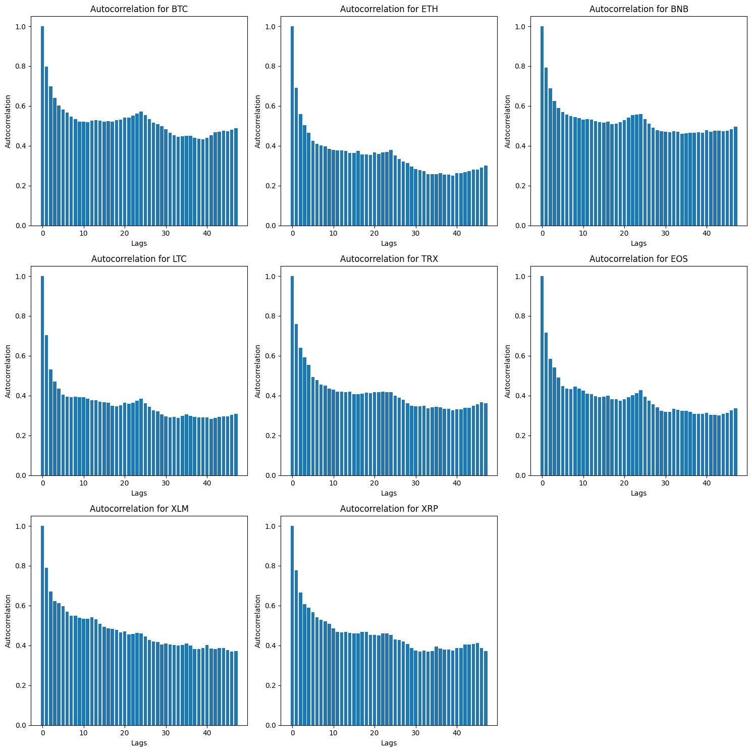
    def create_autocorrelation_plots(self, nlags: Optional[int] = None):
        """
        Creates autocorrelation plots for the trading volume of specified assets.

        Args:
        nlags (int, optional): The number of lags to be used in the autocorrelation plots.
        """
        self._initialize_plot()
        for i, asset in enumerate(self.assets):
            series = self.data[f'{asset} volume']
            autocorr = [series.autocorr(lag) for lag in range(nlags)]

            self.axs[i].bar(range(nlags), autocorr)
            self._set_plot_details(i, f'Autocorrelation for {asset}', 'Lags', 'Autocorrelation')

        self._finalize_plot()


    def create_market_share_plots(self):
        """
        Creates plots visualizing market share changes during different global market hours.
        """
        market_shares = self._compute_market_shares()
        self._initialize_plot()

        for i, asset in enumerate(self.assets):
            market_hours_data = market_shares[asset].groupby(market_shares.index.hour).mean()
            market_hours_data.plot(ax=self.axs[i], kind='bar', title=f'Market Share During Hours for {asset}')
            self._set_plot_details(i, f'Market Share During Hours for {asset}', 'Hour of Day', 'Average Market Share')
            MarketHour.apply_shading(self.axs[i])  # Assuming MarketHour.apply_shading is defined elsewhere

        self._finalize_plot()

    def _compute_market_shares(self):
        """
        Computes the market share for each asset based on quote asset volume.
        """
        total_volumes = self.data[[f'{asset} quote asset volume' for asset in self.assets]]
        total_volumes.columns = [c.replace(' quote asset volume', '') for c in total_volumes.columns]
        market_shares = total_volumes.divide(total_volumes.sum(axis=1), axis=0)
        return market_shares


    def _set_plot_details(self, index: int, title: str, xlabel: str, ylabel: str):
        """
        Sets common details for a subplot.

        Args:
        index (int): The index of the subplot in the axs array.
        title (str): The title of the subplot.
        xlabel (str): The label for the x-axis.
        ylabel (str): The label for the y-axis.
        """
        self.axs[index].set_title(title)
        self.axs[index].set_xlabel(xlabel)
        self.axs[index].set_ylabel(ylabel)

    def _finalize_plot(self):
        """
        Finalizes the plot by hiding unused subplots and adjusting the layout.
        """
        for i in range(len(self.assets), len(self.axs)):
            self.axs[i].axis('off')
        plt.tight_layout()
        plt.show()


# Example usage
#visualizer = CryptoDataVisualizer(data, selected_assets)
#visualizer.create_scatter_plots()
#visualizer.create_scatter_plots(True)
#visualizer.create_hourly_seasonality_plots()
#visualizer.create_autocorrelation_plots(48)
#visualizer.create_autocorrelation_plots(7*24*3)
#visualizer.create_autocorrelation_plots(15000)
Creating tools to get statistics about the datas
class CryptoStatsAnalyzer:
    def __init__(self, data: pd.DataFrame, assets: List[str]):
        """
        Initializes the CryptoStatsAnalyzer with cryptocurrency data and a list of assets.

        Args:
        data (pd.DataFrame): The dataset containing cryptocurrency information.
        assets (List[str]): List of assets to analyze.
        """
        self.data = data
        self.assets = assets


    def analyze_returns(self) -> pd.DataFrame:
        stats_summary = pd.DataFrame()

        for asset in self.assets:
            returns = (self.data[f'{asset} close'] / self.data[f'{asset} close'].shift() -1).dropna()
            jb_stat, jb_pvalue = jarque_bera(returns)
            sw_stat, sw_pvalue = shapiro(returns)
            skewness = returns.skew()
            kurtosis = returns.kurtosis()

            # Interpretations
            normality_interpretation = self._interpret_normality(jb_pvalue, sw_pvalue)
            risk_interpretation = self._interpret_risk(skewness, kurtosis)

            asset_stats = {
                'Mean': returns.mean(),
                'Std Dev': returns.std(),
                'Skewness': skewness,
                'Kurtosis': kurtosis,
                'Jarque-Bera Stat': jb_stat,
                'Jarque-Bera P-Value': jb_pvalue,
                'Shapiro-Wilk Stat': sw_stat,
                'Shapiro-Wilk P-Value': sw_pvalue,
                'Normality Interpretation': normality_interpretation,
                'Risk Interpretation': risk_interpretation
            }

            stats_summary[asset] = pd.Series(asset_stats)

        return stats_summary.transpose()

    def _interpret_normality(self, jb_pvalue: float, sw_pvalue: float) -> str:
        if jb_pvalue < 0.05 and sw_pvalue < 0.05:
            return "Likely not normal distribution"
        return "Possibly normal distribution"

    def _interpret_risk(self, skewness: float, kurtosis: float) -> str:
        if skewness > 1 or skewness < -1:
            skewness_risk = "High skewness (potential risk)"
        else:
            skewness_risk = "Low skewness"

        if kurtosis > 3:
            kurtosis_risk = "High kurtosis (heavy tails)"
        else:
            kurtosis_risk = "Low kurtosis"

        return f"{skewness_risk}, {kurtosis_risk}"


    def analyze_market_share(self):
        """
        Performs a comprehensive market share analysis based on quote asset volume,
        including standard deviation, quantile analysis, and market hour impact.
        """
        # Compute market shares
        market_shares = self._compute_market_shares()


        # Analyze standard deviation and quantiles
        market_share_stats = pd.DataFrame()
        for asset in self.assets:
            asset_volumes = self.data[f'{asset} quote asset volume']
            market_share_stats[asset] = {
                'Mean Market Share': market_shares[asset].mean(),
                'Market Share Std Dev': market_shares[asset].std(),
                '10% Quantile': market_shares[asset].quantile(0.1)
            }

        return market_share_stats

    def _compute_market_shares(self):
        """
        Computes the market share for each asset based on quote asset volume.
        """
        total_volumes = self.data[[f'{asset} quote asset volume' for asset in self.assets]]
        total_volumes.columns = [c[:-len(' quote asset volume')] for c in total_volumes.columns]
        market_shares = total_volumes.divide(total_volumes.sum(axis=1), axis=0)
        return market_shares


# Example usage
#stats_analyzer = CryptoStatsAnalyzer(data, selected_assets)
#returns_stats = stats_analyzer.analyze_returns()
#print(returns_stats)
#volume_shares = stats_analyzer.analyze_market_share()
# Manually Select a Representative Subset of Assets
selected_assets: List[str] = ["BTC", "ETH", "BNB", "LTC", "TRX", "EOS", "XLM", "XRP"]  # Example selection
# For launching on all assets: selected_assets = final_assets
#selected_assets = [asset for asset in final_assets if asset not in ['COCOS']]
# Detailed Analysis for Selected Assets
selected_data = data[[col for col in data.columns if any(asset in col for asset in selected_assets)]]

# Initialize Visualizer and Analyzer Classes
visualizer = CryptoDataVisualizer(data, selected_assets)
stats_analyzer = CryptoStatsAnalyzer(data, selected_assets)

# Correlation Heatmap of All Assets (Closing Prices)
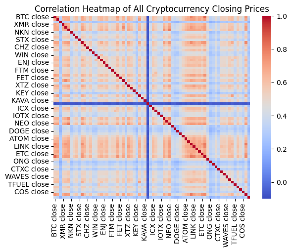
print("\n--- Correlation Heatmap of All Cryptocurrency Closing Prices ---")
all_close_prices = data[[col for col in data.columns if 'close' in col]]
all_close_returns = (all_close_prices / all_close_prices.shift() - 1).dropna()
correlation_matrix_all = all_close_returns.corr()
sns.heatmap(correlation_matrix_all, annot=False, cmap='coolwarm')
plt.title('Correlation Heatmap of All Cryptocurrency Closing Prices')
plt.show()

# Volatility Analysis for Selected Assets
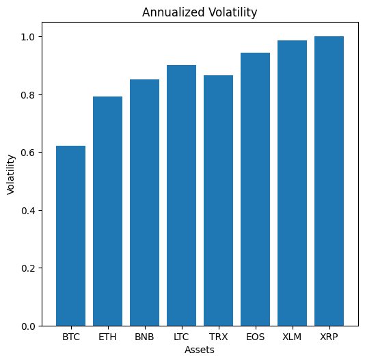
print("\n--- Volatility Analysis for Selected Cryptocurrencies ---")
visualizer.create_volatility_plots()

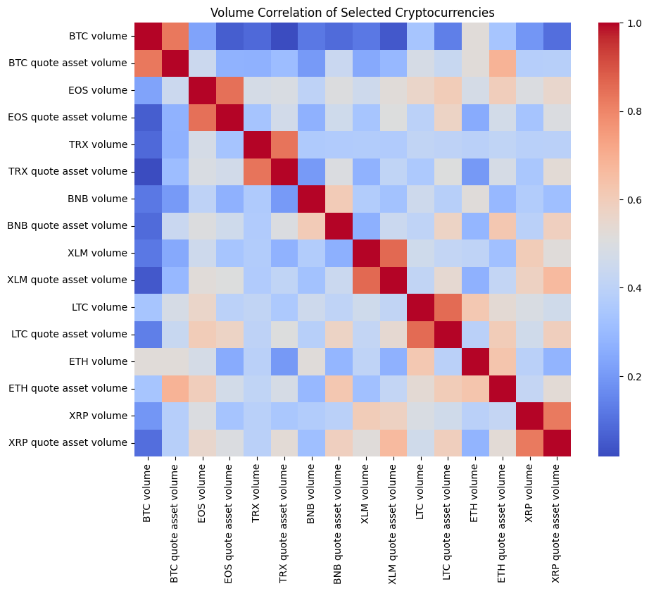
# Heatmap of Volume Correlations for Selected Assets
selected_volumes = selected_data[[col for col in selected_data.columns if 'volume' in col]]
volume_correlation = selected_volumes.corr()
plt.figure(figsize=(10, 8))
sns.heatmap(volume_correlation, annot=False, cmap='coolwarm')
plt.title('Volume Correlation of Selected Cryptocurrencies')
plt.show()

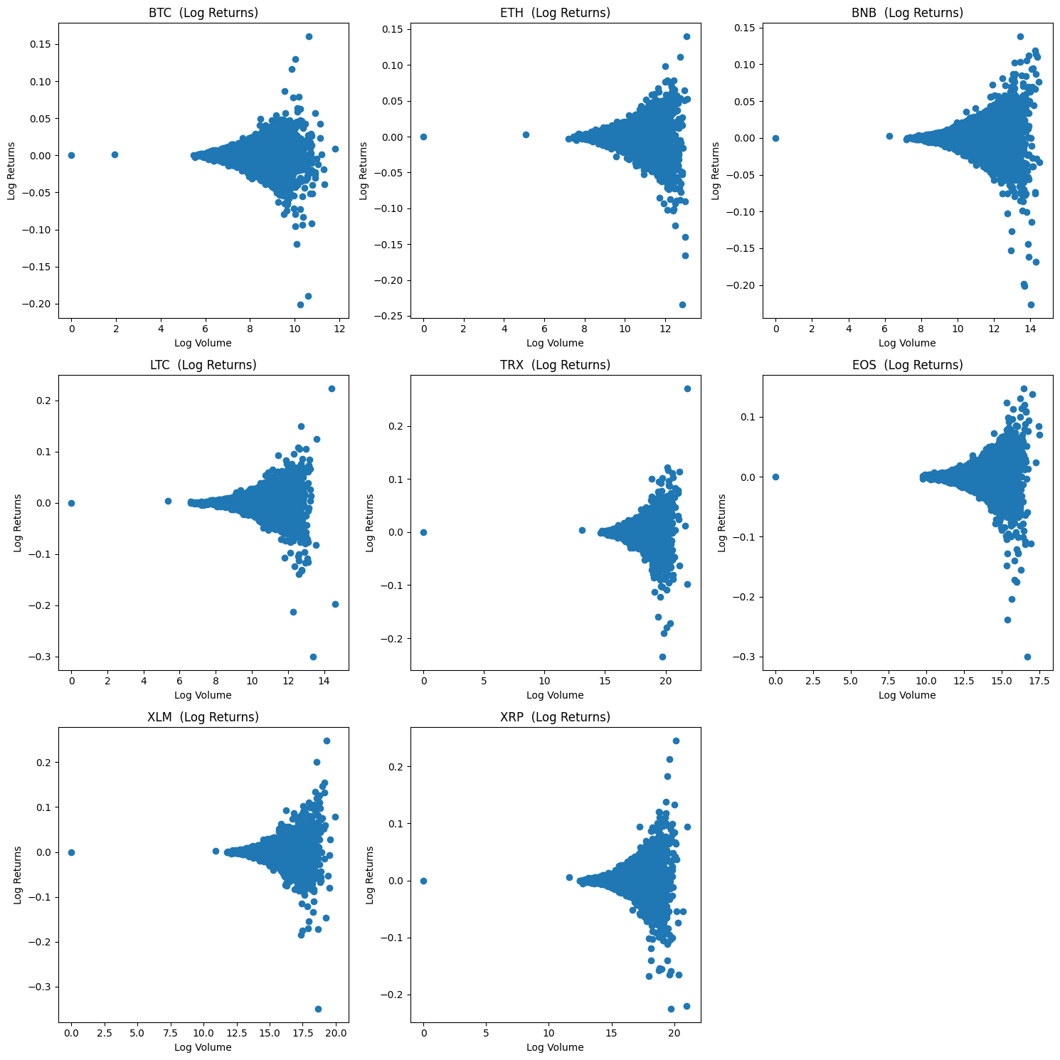
# Scatter Plot of Log Volumes vs. Log Returns for Selected Assets
print("\n--- Scatter Plot of Log Volumes vs. Log Returns for Selected Cryptocurrencies ---")
visualizer.create_scatter_plots()

# Autocorrellogram for Selected Assets
print("\n--- Autocorrelation of Trading Volume for Selected Cryptocurrencies ---")
visualizer.create_autocorrelation_plots(nlags=48)  # Example: 48 lags

# Hourly Seasonality in Volumes for Selected Assets
print("\n--- Hourly Trading Volume for Selected Cryptocurrencies ---")
visualizer.create_hourly_seasonality_plots()

# Statistical Analysis of Returns
print("\n--- Statistical Analysis of Reurns for Selected Cryptocurrencies ---")
return_stats = stats_analyzer.analyze_returns()
print(return_stats)

# Market Share Analysis
print("\n--- Market Share Analysis ---")
visualizer.create_market_share_plots()
market_share_stats = stats_analyzer.analyze_market_share()
print(market_share_stats)

# Additional Statistical Analysis of Market Share (To be implemented)
print("\n--- Additional Statistical Analysis of Market Share ---")
# Additional analysis of market share (e.g., concentration measures, comparison over time, etc.)
--- Correlation Heatmap of All Cryptocurrency Closing Prices ---

--- Volatility Analysis for Selected Cryptocurrencies ---

--- Scatter Plot of Log Volumes vs. Log Returns for Selected Cryptocurrencies ---

--- Autocorrelation of Trading Volume for Selected Cryptocurrencies ---

--- Hourly Trading Volume for Selected Cryptocurrencies ---

--- Statistical Analysis of Reurns for Selected Cryptocurrencies ---
         Mean   Std Dev  Skewness   Kurtosis Jarque-Bera Stat  \
BTC  0.000061  0.008004 -0.462572  44.123182   2170053.096361
ETH   0.00013   0.01019 -0.606696  20.811353    484189.877935
BNB   0.00016   0.01094 -0.547337  28.250765    890544.208508
LTC  0.000086  0.011603 -0.416209  33.831922   1276029.399652
TRX   0.00011  0.011122  0.238046  46.476429   2406894.617438
EOS  0.000032   0.01213 -0.815291  31.379057   1100006.395347
XLM  0.000091  0.012681  0.307561  40.708948   1846819.002676
XRP  0.000095  0.012863  0.354846  36.100442   1452572.056905

    Jarque-Bera P-Value Shapiro-Wilk Stat Shapiro-Wilk P-Value  \
BTC                 0.0           0.82049                  0.0
ETH                 0.0           0.87036                  0.0
BNB                 0.0          0.826394                  0.0
LTC                 0.0          0.854785                  0.0
TRX                 0.0          0.810254                  0.0
EOS                 0.0          0.818779                  0.0
XLM                 0.0          0.823457                  0.0
XRP                 0.0          0.785991                  0.0

           Normality Interpretation                        Risk Interpretation
BTC  Likely not normal distribution  Low skewness, High kurtosis (heavy tails)
ETH  Likely not normal distribution  Low skewness, High kurtosis (heavy tails)
BNB  Likely not normal distribution  Low skewness, High kurtosis (heavy tails)
LTC  Likely not normal distribution  Low skewness, High kurtosis (heavy tails)
TRX  Likely not normal distribution  Low skewness, High kurtosis (heavy tails)
EOS  Likely not normal distribution  Low skewness, High kurtosis (heavy tails)
XLM  Likely not normal distribution  Low skewness, High kurtosis (heavy tails)
XRP  Likely not normal distribution  Low skewness, High kurtosis (heavy tails)

--- Market Share Analysis ---
                           BTC       ETH       BNB       LTC       TRX  \
Mean Market Share     0.544708  0.243032  0.073606  0.024721  0.023888
Market Share Std Dev  0.157592  0.104223  0.058757  0.021241  0.027489
10% Quantile          0.354203  0.106571  0.016137  0.005731  0.004759

                           EOS       XLM       XRP
Mean Market Share     0.019558  0.010062  0.060423
Market Share Std Dev  0.020975  0.015270  0.054911
10% Quantile          0.002119  0.001101  0.017634

--- Additional Statistical Analysis of Market Share ---
/home/remi/.local/lib/python3.11/site-packages/scipy/stats/_morestats.py:1882: UserWarning: p-value may not be accurate for N > 5000.
warnings.warn("p-value may not be accurate for N > 5000.")
/home/remi/.local/lib/python3.11/site-packages/scipy/stats/_morestats.py:1882: UserWarning: p-value may not be accurate for N > 5000.
warnings.warn("p-value may not be accurate for N > 5000.")
/home/remi/.local/lib/python3.11/site-packages/scipy/stats/_morestats.py:1882: UserWarning: p-value may not be accurate for N > 5000.
warnings.warn("p-value may not be accurate for N > 5000.")
/home/remi/.local/lib/python3.11/site-packages/scipy/stats/_morestats.py:1882: UserWarning: p-value may not be accurate for N > 5000.
warnings.warn("p-value may not be accurate for N > 5000.")
/home/remi/.local/lib/python3.11/site-packages/scipy/stats/_morestats.py:1882: UserWarning: p-value may not be accurate for N > 5000.
warnings.warn("p-value may not be accurate for N > 5000.")
/home/remi/.local/lib/python3.11/site-packages/scipy/stats/_morestats.py:1882: UserWarning: p-value may not be accurate for N > 5000.
warnings.warn("p-value may not be accurate for N > 5000.")
/home/remi/.local/lib/python3.11/site-packages/scipy/stats/_morestats.py:1882: UserWarning: p-value may not be accurate for N > 5000.
warnings.warn("p-value may not be accurate for N > 5000.")
/home/remi/.local/lib/python3.11/site-packages/scipy/stats/_morestats.py:1882: UserWarning: p-value may not be accurate for N > 5000.
warnings.warn("p-value may not be accurate for N > 5000.")Splitting into train and test
In order to compare the next methods on an OOS part, we will cut our dataset in two parts
final_assets = [asset for asset in final_assets if asset not in ['COCOS', 'BUSD']]cut = int(len(data) * 0.5)
data_train, data_test = data.iloc[:cut], data.iloc[cut:]Standard Markowitz Portfolio Optimization
Solving the Markowitz Optimization Problem
The Optimization Problem
The Markowitz model seeks to find the optimal portfolio that offers the maximum expected return for a given level of risk, or the minimum risk for a given level of expected return. Mathematically, this involves optimizing a function that represents either the portfolio’s expected return or its risk (variance).
Common Methods for Solving
Analytical Methods: Involves using mathematical formulas and constraints to find the optimal portfolio weights. This method can be complex due to the nonlinear nature of the optimization problem.
Quadratic Programming: A popular method for solving the Markowitz model, as the problem can be formulated as a quadratic programming problem. This involves minimizing a quadratic objective function (portfolio variance) subject to linear constraints (like budget constraint and return targets).
Monte Carlo Simulation: Involves simulating a large number of possible portfolios and selecting the one that offers the best risk-return trade-off. This method is useful when the asset returns are not normally distributed or when the optimization problem is highly complex.
Detailed Analytical Solution of Markowitz Optimization
When solving the Markowitz portfolio optimization problem analytically in the global (unconstrained) case, the key is to use a Lagrangian function that takes into account the constraints of the problem. Below is a detailed explanation of this process.
Formulating the Optimization Problem
Consider a portfolio of $ N $ assets. The goal is to minimize the portfolio variance (a measure of risk), subject to the constraint that the total weight of the portfolio equals 1 (full investment of the portfolio budget). The expected return of the portfolio is not fixed but a parameter that will change along the efficient frontier.
Parameters
- Let $ R = (R_1, R_2, , R_N) $ be the vector of expected returns for the ( N ) assets.
- Let $ $ be the covariance matrix of the asset returns.
- Let $ w = (w_1, w_2, , w_N) $ be the vector of weights of the assets in the portfolio.
Objective Function
The objective is to minimize the portfolio variance, given by $ w^w $ (where $ w^$ denotes the transpose of $ w $).
Constraint
The sum of the weights must equal 1, i.e., $ _{i=1}^{N} w_i = 1 $.
The Lagrangian Method
To solve this constrained optimization problem, we introduce a Lagrange multiplier $ $ and construct the Lagrangian function $ L(w, ) $:
\[ L(w, \lambda) = w^\top \Sigma w - \lambda \left( \sum_{i=1}^{N} w_i - 1 \right) \]
Solving the Optimization Problem
- Differentiate the Lagrangian: Compute the partial derivatives of $ L $ with respect to each $ w_i $ and $ $.
- Set the Derivatives to Zero: This yields a system of linear equations.
- Solve the Linear System: Solving this system gives the optimal weights $ w $ for the minimum variance portfolio.
Specific Steps:
- For each $ w_i $, $ = 2 {j=1}^{N} {ij} w_j - = 0 $.
- Additionally, $ = _{i=1}^{N} w_i - 1 = 0 $.
- Solving this set of $ N + 1 $ equations will yield the optimal weights.
Limitations with Long-Only Constraint
In the case of a long-only constraint (where each $ w_i $), the problem becomes a Quadratic Programming problem. The analytical method described above does not directly apply because the non-negativity constraints on the weights complicate the solution. This constraint can lead to a situation where the global minimum variance portfolio contains short positions, which are not allowed under the long-only constraint.
Reconsidering the Use of Monte Carlo Simulation in Portfolio Optimization
When approaching portfolio optimization, especially in the context of cryptocurrency assets, there is a common inclination to favor Monte Carlo Simulation, primarily due to its flexibility and perceived universal applicability. However, this section aims to reassess this preference, highlighting the challenges and limitations of relying solely on Monte Carlo Simulation, particularly when dealing with a large number of assets.
Limitations of Monte Carlo Simulation with Many Assets
Increased Computational Demand: The efficiency of Monte Carlo Simulation deteriorates as the number of assets increases. With each additional asset, the number of required simulations to explore the entire space of possible portfolios grows exponentially. This exponential growth leads to significant increases in computational time and resource requirements.
Difficulty in Finding Optimal Solutions: In scenarios with many assets, the sheer volume of potential portfolio combinations makes it increasingly challenging for Monte Carlo Simulation to reliably find the optimal solution. The probability of sampling the optimal or near-optimal portfolios decreases as the search space expands.
Practical Feasibility: For portfolios with a large number of assets, the computational burden can render Monte Carlo Simulation nearly unfeasible in practice. This is particularly relevant in real-world scenarios where timely decision-making is crucial, and computational resources may be limited.
Comparison with Quadratic Optimization
Quadratic optimization, as a more traditional approach to solving the Markowitz portfolio optimization problem, presents a contrast to Monte Carlo Simulation. While it has its limitations, such as difficulties in handling non-linear constraints and the need for precise estimates of returns and covariances, quadratic optimization can be more efficient and direct in finding the optimal portfolio, especially when the number of assets is large.
Demonstrating with Code
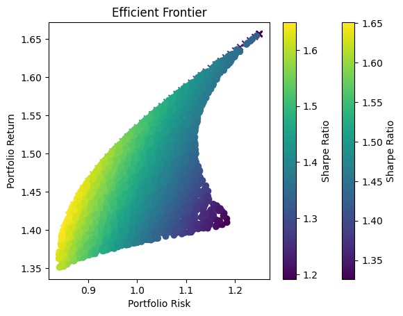
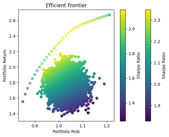
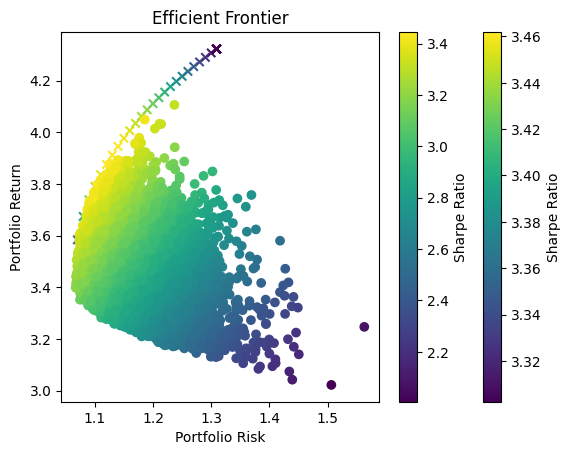
To illustrate these points, code examples can be provided that compare the efficient frontier obtained through quadratic optimization versus Monte Carlo Simulation. These examples can demonstrate how the efficient frontier might differ between the two methods and underscore the potential challenges in using Monte Carlo Simulation for large asset pools.
This comparison not only serves as a practical demonstration but also reinforces the need for a balanced approach in selecting optimization techniques, considering both the nature of the asset pool and the practical constraints of the analysis.
def get_prices(data, assets):
    prices = data[[f'{asset} close' for asset in assets]].ffill()
    #prices.loc[:, 'cash']=1
    return prices

def compute_returns(prices):
    return (prices / prices.shift(1) - 1).iloc[1:]

def portfolio_expected_return(weights, expected_return):
    return weights @ expected_return

def portfolio_annualized_expected_return(weights, expected_return):
    return portfolio_expected_return(weights, expected_return) * 24 * 365

def portfolio_variance(weights, covariance_matrix):
    return weights.T @ covariance_matrix @ weights

def portfolio_annualized_risk(weights, covariance_matrix):
    return np.sqrt(portfolio_variance(weights, covariance_matrix)) * np.sqrt(24*365)

def optimize_portfolio(mu, sigmas, max_volatility):
    num_assets = len(mu)
    args = (mu, sigmas)

    # Objective function to maximize returns
    def objective_function(weights, mu, _):
        return -portfolio_annualized_expected_return(weights, mu)

    # Constraint for the weights to sum up to 1
    constraints = [{'type': 'eq', 'fun': lambda x: np.sum(x) - 1}]

    # Additional constraint for maximum volatility
    constraints.append({'type': 'ineq', 'fun': lambda x: max_volatility - portfolio_annualized_risk(x, sigmas)})

    bounds = tuple((0, 1) for asset in range(num_assets))

    initial_weight = np.array(num_assets * [np.random.random()])
    initial_weight /= sum(initial_weight)

    result = minimize(objective_function, initial_weight, args=args, method='SLSQP', bounds=bounds, constraints=constraints)
    return result


def plot_optimized_efficient_frontier(mu, sigmas, show=True):
    portfolio_means, portfolio_risks = [], []
    for max_volatility in np.arange(0.8, 1.4, 0.01):
        optimization_result = optimize_portfolio(mu, sigmas, max_volatility)
        if optimization_result.success:
            optimal_weights=optimization_result.x
            portfolio_means.append(portfolio_annualized_expected_return(optimal_weights, mu))
            portfolio_risks.append(portfolio_annualized_risk(optimal_weights, sigmas))
    portfolio_means, portfolio_risks = np.array(portfolio_means), np.array(portfolio_risks)
    plt.scatter(portfolio_risks, portfolio_means, c=portfolio_means/portfolio_risks, marker='x')
    plt.title('Efficient Frontier')
    plt.xlabel('Portfolio Risk')
    plt.ylabel('Portfolio Return')
    plt.colorbar(label='Sharpe Ratio')
    if show:
        plt.show()

# Function to plot the efficient frontier
def plot_monte_carlo_only_efficient_frontier(mu, sigmas, num_portfolios=10000, show=True):
    num_assets = len(mu)
    portfolio_means, portfolio_risks = [], []

    for _ in range(num_portfolios):
        weights = np.random.random(num_assets)
        weights /= np.sum(weights)
        portfolio_means.append(portfolio_annualized_expected_return(weights, mu))
        portfolio_risks.append(portfolio_annualized_risk(weights, sigmas))
    portfolio_means, portfolio_risks = np.array(portfolio_means), np.array(portfolio_risks)
    plt.scatter(portfolio_risks, portfolio_means, c=portfolio_means/portfolio_risks, marker='o')
    plt.title('Efficient Frontier')
    plt.xlabel('Portfolio Risk')
    plt.ylabel('Portfolio Return')
    plt.colorbar(label='Sharpe Ratio')
    if show:
        plt.show()


def print_stats(prices, ptf_name):
    returns = (prices / prices.shift(1) - 1).iloc[1:]
    print(f'{ptf_name} has an expected return of {returns.mean() * 365 * 24} for a risk of {returns.std() * np.sqrt(365*24)}')
maximum_volatility = 1.1
for selected_assets in [['BTC', 'TRX', 'LTC'], ["BTC", "ETH", "BNB", "LTC", "TRX", "EOS", "XLM", "XRP"], final_assets]:
print(f'Using :{selected_assets}')
prices_train = get_prices(data_train, selected_assets)
returns_train = compute_returns(prices_train)
mu = returns_train.mean().values
sigmas = returns_train.cov().values
plot_optimized_efficient_frontier(mu, sigmas, show=False)
plot_monte_carlo_only_efficient_frontier(mu, sigmas, show=False)
plt.show()
optimization_result = optimize_portfolio(mu, sigmas, maximum_volatility)
if optimization_result.success:
optimal_weights = optimization_result.x
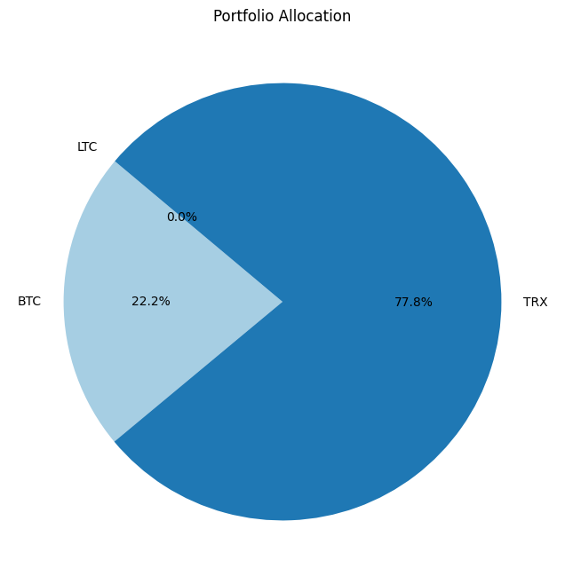
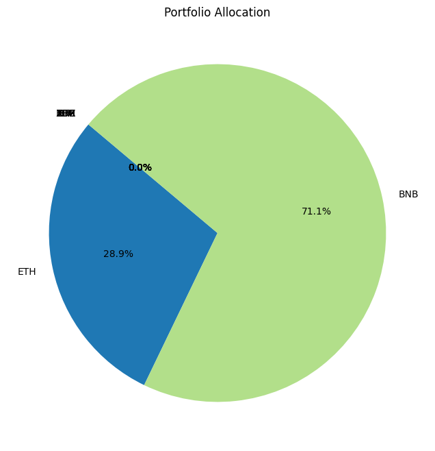
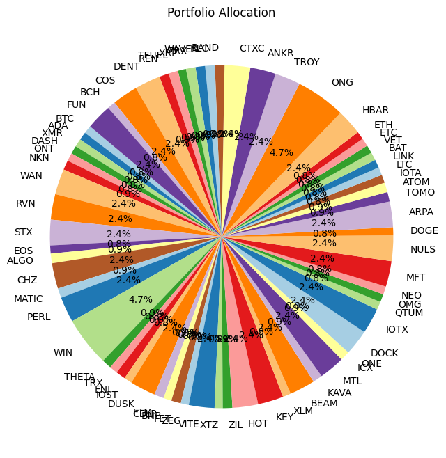
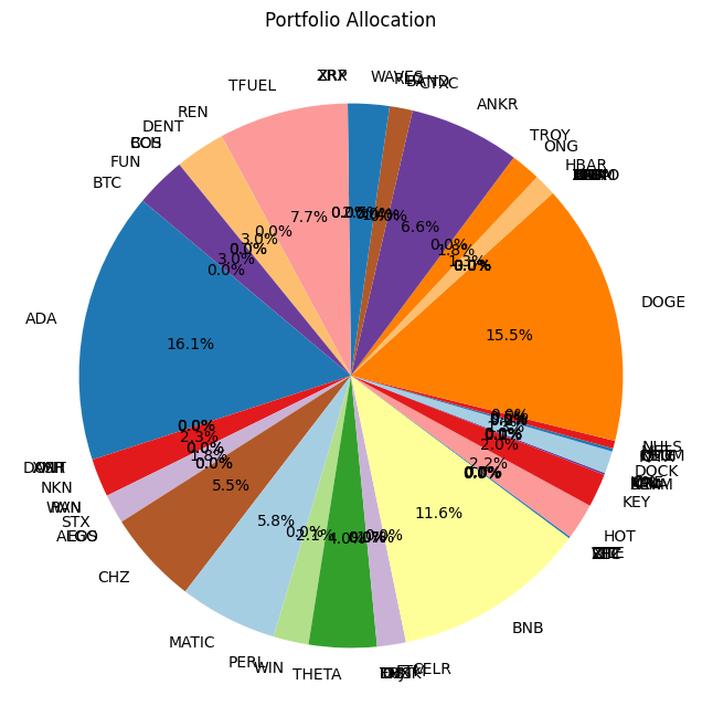
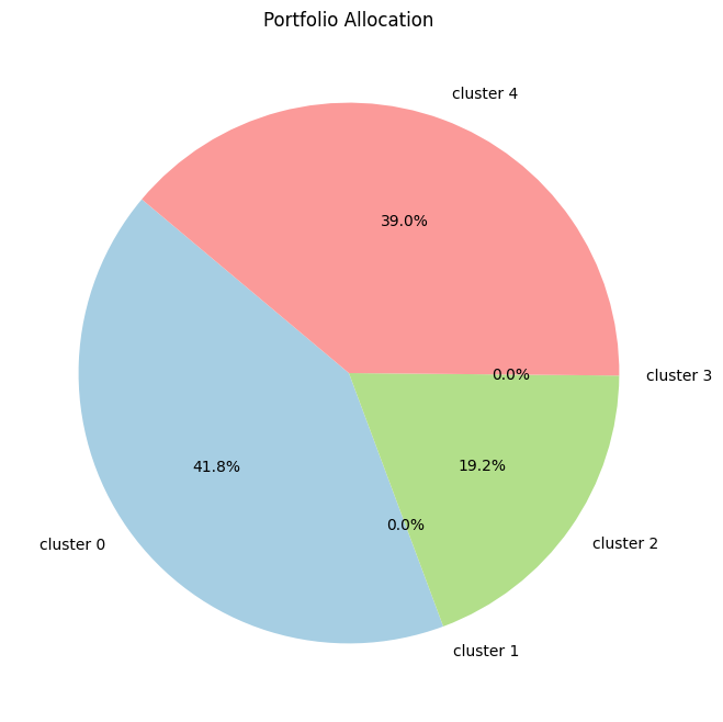
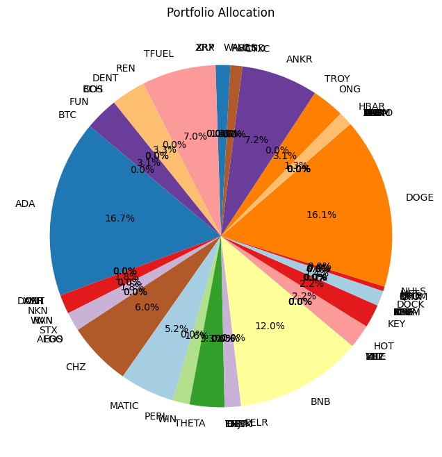
# Create the pie chart
plt.figure(figsize=(8, 8))
plt.pie(optimal_weights, labels=selected_assets, autopct='%1.1f%%', startangle=140, colors=plt.cm.Paired.colors)
# Adding title
plt.title('Portfolio Allocation')
# Show the plot
plt.show()
else:
print("Did not converge")
print('\n'*3)Using :['BTC', 'TRX', 'LTC']
Using :['BTC', 'ETH', 'BNB', 'LTC', 'TRX', 'EOS', 'XLM', 'XRP']
Using :['BTC', 'ADA', 'XMR', 'DASH', 'ONT', 'NKN', 'WAN', 'RVN', 'STX', 'EOS', 'ALGO', 'CHZ', 'MATIC', 'PERL', 'WIN', 'THETA', 'TRX', 'ENJ', 'IOST', 'DUSK', 'FTM', 'CELR', 'BNB', 'FET', 'ZEC', 'VITE', 'XTZ', 'ZIL', 'HOT', 'KEY', 'XLM', 'BEAM', 'KAVA', 'MTL', 'ICX', 'ONE', 'DOCK', 'IOTX', 'QTUM', 'OMG', 'NEO', 'MFT', 'NULS', 'DOGE', 'ARPA', 'TOMO', 'ATOM', 'IOTA', 'LTC', 'LINK', 'BAT', 'VET', 'ETC', 'ETH', 'HBAR', 'ONG', 'TROY', 'ANKR', 'CTXC', 'BAND', 'RLC', 'WAVES', 'ZRX', 'XRP', 'TFUEL', 'REN', 'DENT', 'COS', 'BCH', 'FUN']
Optimization Method Selection and Asset Scale
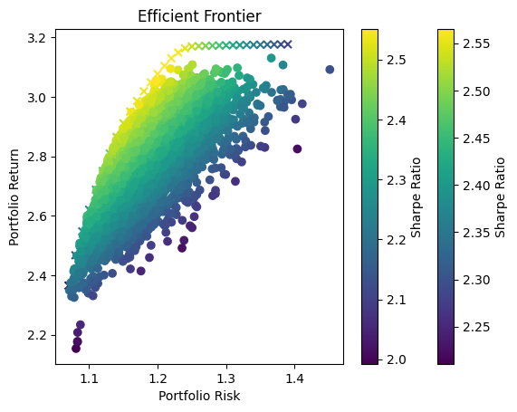
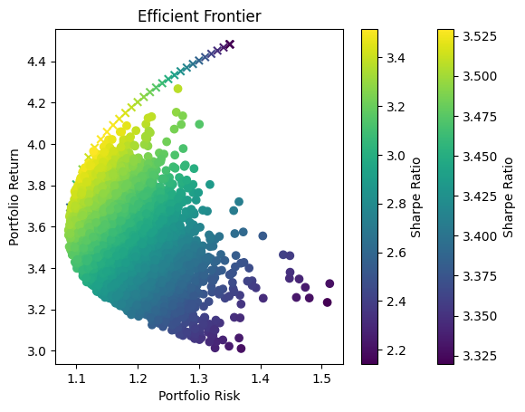
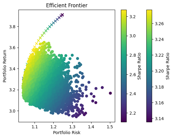
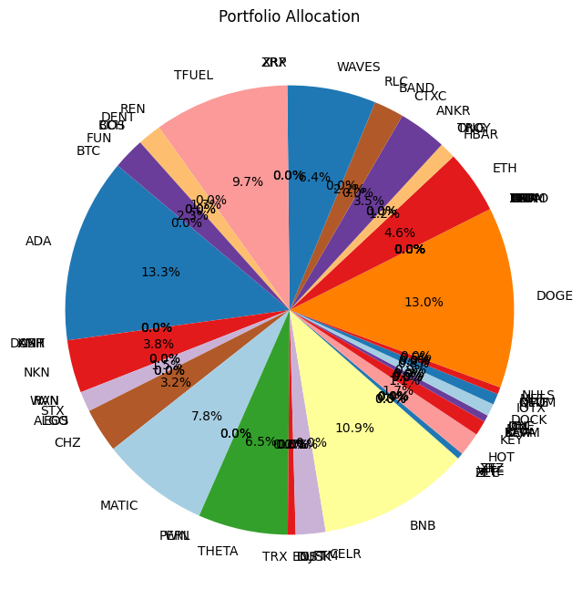
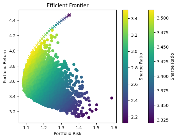
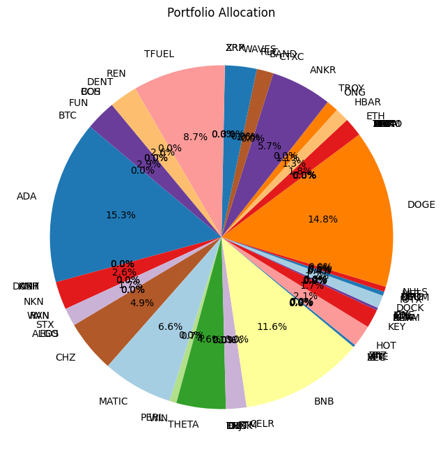
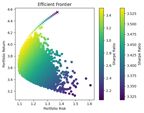
In portfolio optimization, the selection of an appropriate method hinges on the scale and complexity of the asset pool. The charts provided illustrate a crucial point: Monte Carlo Simulation’s suitability diminishes as the number of assets increases. This trend is evident when comparing the efficient frontiers for portfolios with varying numbers of assets—3, 8, and 70.
Monte Carlo Simulation and Large Asset Pools
As observed, with three assets, the efficient frontiers produced by Monte Carlo Simulation and Quadratic Optimization are closely aligned. However, as the number of assets grows to eight, the Monte Carlo frontier becomes less efficient, failing to encompass the optimal risk-return combinations that Quadratic Optimization identifies. This inefficiency is further exacerbated in the 70-asset portfolio, where the Monte Carlo frontier is significantly suboptimal.
Underlying Causes of Inefficiency
This inefficiency stems from the fundamental nature of Monte Carlo Simulation. The method relies on random sampling to approximate the efficient frontier, and as the dimensionality of the problem increases with more assets, the required number of samples to accurately approximate the frontier grows exponentially. Consequently, Monte Carlo Simulation may not adequately sample the vast solution space, leading to a suboptimal representation of the efficient frontier.
Standard Challenges in Portfolio Optimization
The challenges faced with Monte Carlo Simulation in higher-dimensional spaces are not unique but rather a standard problem in computational finance. With increasing assets, the complexity of capturing the interdependencies and risk-return dynamics grows, necessitating more advanced and computationally intensive methods.
Evaluation of the performance - Backtesting In and Out of Sample
Understanding Backtesting in Portfolio Management
Backtesting is a pivotal technique in portfolio management and financial analysis, where historical data is used to simulate the performance of a portfolio strategy or model over a specific period. The primary purpose of backtesting is to evaluate the effectiveness, robustness, and viability of a strategy by observing how it would have behaved in the past. It allows investors and portfolio managers to:
- Assess Strategy Performance: Gauge the potential returns and risks of a strategy before applying it in real-world scenarios.
- Identify Potential Flaws: Uncover issues that may not be apparent through theoretical models, such as overfitting or underperformance during certain market conditions.
- Optimize Strategy Parameters: Fine-tune the parameters of the strategy to improve its future performance based on past outcomes.
- Understand Market Dynamics: Gain insights into how different assets and portfolio compositions respond to market volatility and changes over time.
Backtesting is not without its limitations. It assumes that historical conditions are indicative of future performances, which may not always hold true, especially in dynamic and unpredictable markets like cryptocurrencies. Moreover, it often does not account for transaction costs, market impact, liquidity, or slippage, which can significantly affect real-world returns.
Practical Implications of Portfolio Rebalancing
In the theoretical framework of portfolio optimization, continuous rebalancing is posited as an ideal approach to maintain the optimal risk-return profile. However, in practice, continuous rebalancing is seldom feasible due to the associated costs and market impacts, particularly in the cryptocurrency space. Instead, portfolios are often rebalanced on a more periodic basis—quarterly, semi-annually, or annually.
Trading Costs in Cryptocurrency Markets
Cryptocurrency markets are known for their high volatility and often substantial bid-ask spreads. This can lead to considerable trading costs, including:
- Spread Costs: The difference between the buying price and the selling price of an asset can be wide, especially for less liquid assets.
- Slippage: The price at which a trade is executed can differ from the expected price, particularly for large orders or during periods of high volatility.
- Transaction Fees: Exchanges and trading platforms may charge fees for each transaction, which can accumulate with frequent trading.
These factors combined make the cost of continuous rebalancing prohibitive. Instead, a more measured approach to rebalancing must be adopted—one that balances the benefits of maintaining an optimal portfolio composition with the real costs of executing trades.
In sample
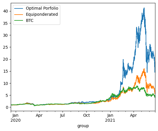
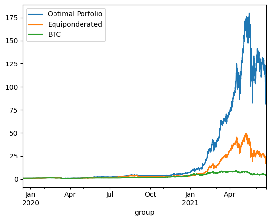
Backtesting case 1 - continuous reponderation
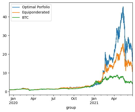
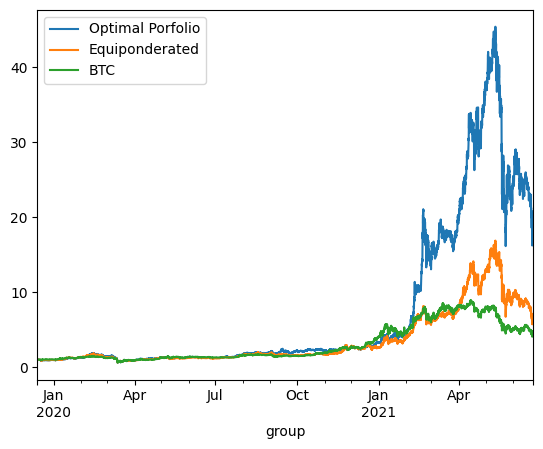
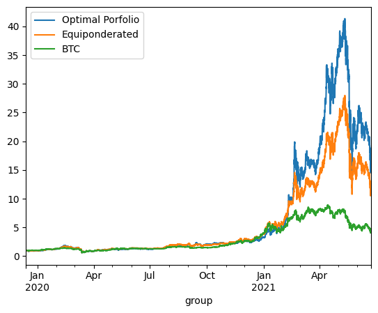
maximum_volatility = 1.1

for selected_assets in [['BTC', 'ETH', 'BNB'], ["BTC", "ETH", "BNB", "LTC", "TRX", "EOS", "XLM", "XRP"], final_assets]:

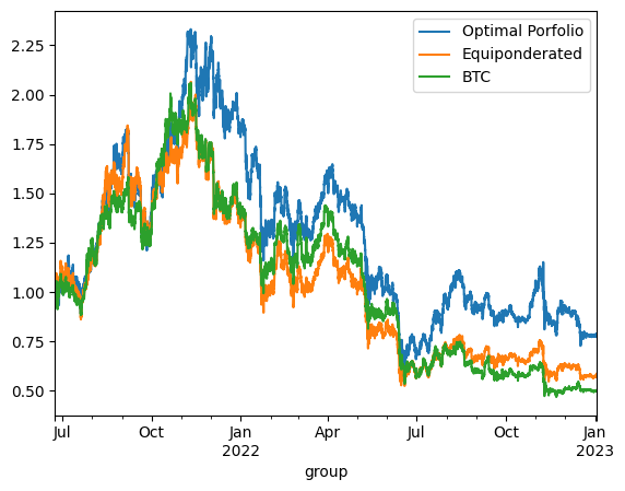
    print('On Train using continuous reponderation:')
    prices = get_prices(data_train, selected_assets)
    returns = compute_returns(prices)
    mu = returns.mean()
    sigmas = returns.cov()

    optimization_result = optimize_portfolio(mu, sigmas, maximum_volatility)
    if optimization_result.success:
        optimal_weights = optimization_result.x
        equal_weight = np.ones(prices.shape[1]) / prices.shape[1]
        btc_only_weights = np.array([1 if 'BTC' in c else 0 for c in prices.columns])

        optimized_porfolio_returns = (returns * optimal_weights).sum(axis=1)
        equiponderated_porfolio_returns = (returns * equal_weight).sum(axis=1)
        btc_only_porfolio_returns = (returns * btc_only_weights).sum(axis=1)

        optimized_porfolio_value = (optimized_porfolio_returns +1 ).cumprod()
        equiponderated_porfolio_value = (equiponderated_porfolio_returns + 1).cumprod()
        btc_only_porfolio_value = (btc_only_porfolio_returns + 1).cumprod()

        optimized_porfolio_value.plot(label='Optimal Porfolio')
        equiponderated_porfolio_value.plot(label='Equiponderated')
        btc_only_porfolio_value.plot(label='BTC')
        plt.legend()
        plt.show()

        print_stats(optimized_porfolio_value, "optimized_porfolio_value")
        print_stats(equiponderated_porfolio_value, "equiponderated_porfolio_value")
        print_stats(btc_only_porfolio_value, "btc_only_porfolio_value")
    else:
        print("Did not converge")

    print('\n'*3)
On Train using continuous reponderation:
optimized_porfolio_value has an expected return of 2.548151418247148 for a risk of 1.1000340646158004
equiponderated_porfolio_value has an expected return of 2.0884018962457334 for a risk of 0.9415126546710327
btc_only_porfolio_value has an expected return of 1.3450136751201247 for a risk of 0.8411451768924758
On Train using continuous reponderation:
optimized_porfolio_value has an expected return of 2.5481514168584285 for a risk of 1.1000340635856367
equiponderated_porfolio_value has an expected return of 1.7604502330310838 for a risk of 1.016501173754713
btc_only_porfolio_value has an expected return of 1.3450136751201247 for a risk of 0.8411451768924758
On Train using continuous reponderation:
optimized_porfolio_value has an expected return of 3.925543641491842 for a risk of 1.1000409259938504
equiponderated_porfolio_value has an expected return of 2.571030019068987 for a risk of 1.1033719694757085
btc_only_porfolio_value has an expected return of 1.3450136751201247 for a risk of 0.8411451768924758
Backtesting case 2 - Ponderation at starting date
maximum_volatility = 1.1

for selected_assets in [['BTC', 'ETH', 'BNB'], ["BTC", "ETH", "BNB", "LTC", "TRX", "EOS", "XLM", "XRP"], final_assets]:

    print('On Train using ponderation at t=0:')
    prices = get_prices(data_train, selected_assets)
    returns = compute_returns(prices)
    mu = returns.mean()
    sigmas = returns.cov()

    optimization_result = optimize_portfolio(mu, sigmas, maximum_volatility)
    if optimization_result.success:
        optimal_weights = optimization_result.x
        equal_weight = np.ones(prices.shape[1]) / prices.shape[1]
        btc_only_weights = np.array([1 if 'BTC' in c else 0 for c in prices.columns])

        optimized_porfolio_value = (prices / prices.iloc[0] * optimal_weights).sum(axis=1)
        equiponderated_porfolio_value = (prices / prices.iloc[0] * equal_weight).sum(axis=1)
        btc_only_porfolio_value = (prices / prices.iloc[0] * btc_only_weights).sum(axis=1)

        optimized_porfolio_returns = (optimized_porfolio_value / optimized_porfolio_value.shift() - 1)
        equiponderated_porfolio_returns = (equiponderated_porfolio_value / equiponderated_porfolio_value.shift() - 1)
        btc_only_porfolio_returns = (btc_only_porfolio_value / btc_only_porfolio_value.shift() - 1)

        optimized_porfolio_value.plot(label='Optimal Porfolio')
        equiponderated_porfolio_value.plot(label='Equiponderated')
        btc_only_porfolio_value.plot(label='BTC')
        plt.legend()
        plt.show()

        print_stats(optimized_porfolio_value, "optimized_porfolio_value")
        print_stats(equiponderated_porfolio_value, "equiponderated_porfolio_value")
        print_stats(btc_only_porfolio_value, "btc_only_porfolio_value")
    else:
        print("Did not converge")

    print('\n'*3)
On Train using ponderation at t=0:
optimized_porfolio_value has an expected return of 2.4989334636751925 for a risk of 1.1143620398195824
equiponderated_porfolio_value has an expected return of 2.148641545657201 for a risk of 0.9987963805734758
btc_only_porfolio_value has an expected return of 1.3475412196303846 for a risk of 0.8411195887632472
On Train using ponderation at t=0:
optimized_porfolio_value has an expected return of 2.4989334620588894 for a risk of 1.1143620390216151
equiponderated_porfolio_value has an expected return of 1.7637480055378254 for a risk of 1.0254619878752895
btc_only_porfolio_value has an expected return of 1.3475412196303846 for a risk of 0.8411195887632472
On Train using ponderation at t=0:
optimized_porfolio_value has an expected return of 3.580661899998042 for a risk of 1.3224220062235903
equiponderated_porfolio_value has an expected return of 2.3591193232677545 for a risk of 1.174243796499045
btc_only_porfolio_value has an expected return of 1.3475412196303846 for a risk of 0.8411195887632472
Out of sample
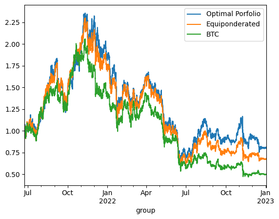
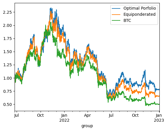
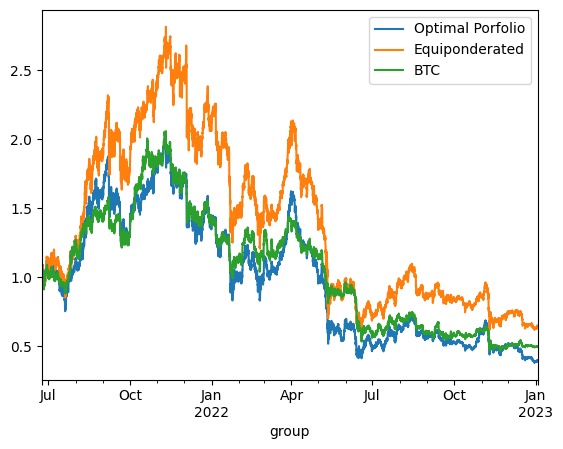
Backtesting case 1 - continuous reponderation
maximum_volatility = 1.1

for selected_assets in [['BTC', 'ETH', 'BNB'], ["BTC", "ETH", "BNB", "LTC", "TRX", "EOS", "XLM", "XRP"], final_assets]:
    prices = get_prices(data_train, selected_assets)
    returns = compute_returns(prices)
    mu = returns.mean()
    sigmas = returns.cov()
    optimization_result = optimize_portfolio(mu, sigmas, maximum_volatility)

    print('On Test using continuous reponderation:')
    prices = get_prices(data_test, selected_assets)
    returns = compute_returns(prices)
    mu = returns.mean()
    sigmas = returns.cov()
    if optimization_result.success:
        optimal_weights = optimization_result.x
        equal_weight = np.ones(prices.shape[1]) / prices.shape[1]
        btc_only_weights = np.array([1 if 'BTC' in c else 0 for c in prices.columns])

        optimized_porfolio_returns = (returns * optimal_weights).sum(axis=1)
        equiponderated_porfolio_returns = (returns * equal_weight).sum(axis=1)
        btc_only_porfolio_returns = (returns * btc_only_weights).sum(axis=1)

        optimized_porfolio_value = (optimized_porfolio_returns +1 ).cumprod()
        equiponderated_porfolio_value = (equiponderated_porfolio_returns + 1).cumprod()
        btc_only_porfolio_value = (btc_only_porfolio_returns + 1).cumprod()

        optimized_porfolio_value.plot(label='Optimal Porfolio')
        equiponderated_porfolio_value.plot(label='Equiponderated')
        btc_only_porfolio_value.plot(label='BTC')
        plt.legend()
        plt.show()

        print_stats(optimized_porfolio_value, "optimized_porfolio_value")
        print_stats(equiponderated_porfolio_value, "equiponderated_porfolio_value")
        print_stats(btc_only_porfolio_value, "btc_only_porfolio_value")
    else:
        print("Did not converge")

    print('\n'*3)
On Test using continuous reponderation:
optimized_porfolio_value has an expected return of 0.15428195025687122 for a risk of 0.7729171922879363
equiponderated_porfolio_value has an expected return of -0.0013986837378817088 for a risk of 0.713765650193611
btc_only_porfolio_value has an expected return of -0.24874776856528497 for a risk of 0.6432098891396297
On Test using continuous reponderation:
optimized_porfolio_value has an expected return of 0.1542819497517422 for a risk of 0.7729171922362768
equiponderated_porfolio_value has an expected return of -0.05433377110132012 for a risk of 0.7326415041884127
btc_only_porfolio_value has an expected return of -0.24874776856528497 for a risk of 0.6432098891396297
On Test using continuous reponderation:
optimized_porfolio_value has an expected return of -0.23193963544241336 for a risk of 0.8589603963330816
equiponderated_porfolio_value has an expected return of 0.09317371980719207 for a risk of 0.872321680813382
btc_only_porfolio_value has an expected return of -0.24874776856528497 for a risk of 0.6432098891396297
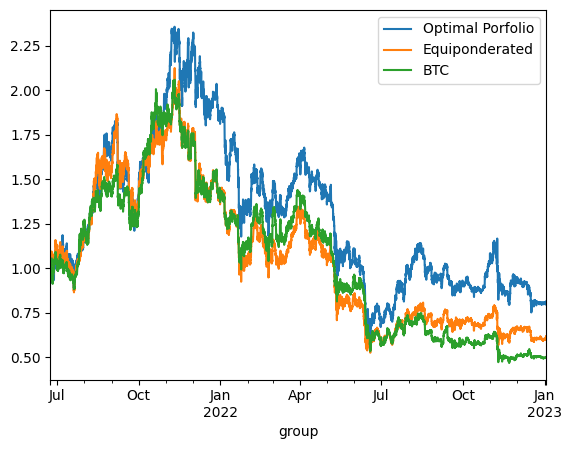
Backtesting case 2 - Ponderation at starting date
maximum_volatility = 1.1

for selected_assets in [['BTC', 'ETH', 'BNB'], ["BTC", "ETH", "BNB", "LTC", "TRX", "EOS", "XLM", "XRP"], final_assets]:

    prices = get_prices(data_train, selected_assets)
    returns = compute_returns(prices)
    mu = returns.mean()
    sigmas = returns.cov()
    optimization_result = optimize_portfolio(mu, sigmas, maximum_volatility)

    print('On Test using ponderation at t=0:')
    prices = get_prices(data_test, selected_assets)
    returns = compute_returns(prices)
    mu = returns.mean()
    sigmas = returns.cov()
    if optimization_result.success:
        optimal_weights = optimization_result.x
        equal_weight = np.ones(prices.shape[1]) / prices.shape[1]
        btc_only_weights = np.array([1 if 'BTC' in c else 0 for c in prices.columns])

        optimized_porfolio_value = (prices / prices.iloc[0] * optimal_weights).sum(axis=1)
        equiponderated_porfolio_value = (prices / prices.iloc[0] * equal_weight).sum(axis=1)
        btc_only_porfolio_value = (prices / prices.iloc[0] * btc_only_weights).sum(axis=1)

        optimized_porfolio_returns = (optimized_porfolio_value / optimized_porfolio_value.shift() - 1)
        equiponderated_porfolio_returns = (equiponderated_porfolio_value / equiponderated_porfolio_value.shift() - 1)
        btc_only_porfolio_returns = (btc_only_porfolio_value / btc_only_porfolio_value.shift() - 1)

        optimized_porfolio_value.plot(label='Optimal Porfolio')
        equiponderated_porfolio_value.plot(label='Equiponderated')
        btc_only_porfolio_value.plot(label='BTC')
        plt.legend()
        plt.show()

        print_stats(optimized_porfolio_value, "optimized_porfolio_value")
        print_stats(equiponderated_porfolio_value, "equiponderated_porfolio_value")
        print_stats(btc_only_porfolio_value, "btc_only_porfolio_value")
    else:
        print("Did not converge")

    print('\n'*3)
On Test using ponderation at t=0:
optimized_porfolio_value has an expected return of 0.1385214791312807 for a risk of 0.7720799071383421
equiponderated_porfolio_value has an expected return of -0.015265894665119857 for a risk of 0.7191928198459694
btc_only_porfolio_value has an expected return of -0.24608407102642182 for a risk of 0.6431943165220202
On Test using ponderation at t=0:
optimized_porfolio_value has an expected return of 0.13852147846267007 for a risk of 0.7720799070715625
equiponderated_porfolio_value has an expected return of -0.09400856892034151 for a risk of 0.7196933806779569
btc_only_porfolio_value has an expected return of -0.24608407102642182 for a risk of 0.6431943165220202
On Test using ponderation at t=0:
optimized_porfolio_value has an expected return of -0.3888911847590084 for a risk of 0.8484406265560269
equiponderated_porfolio_value has an expected return of -0.1894050612562228 for a risk of 0.8925118088027398
btc_only_porfolio_value has an expected return of -0.24608407102642182 for a risk of 0.6431943165220202
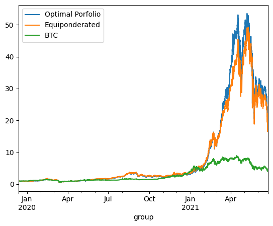
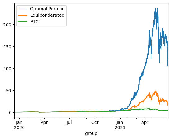
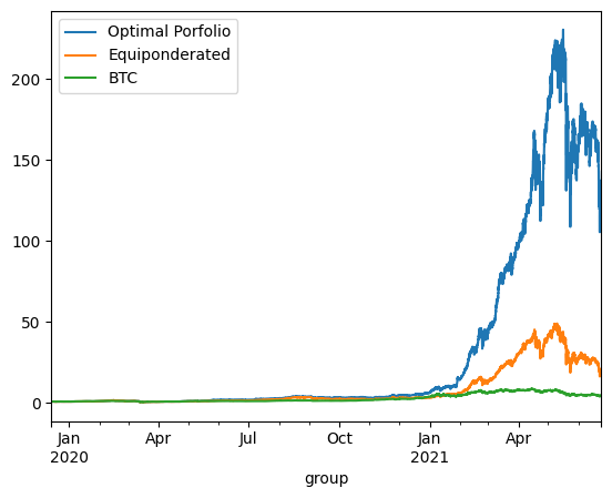
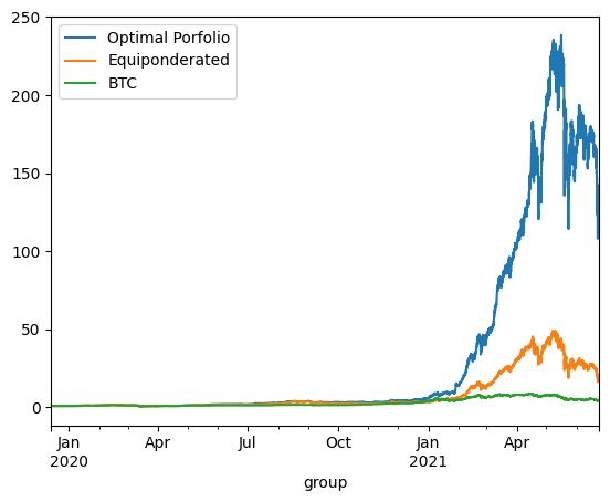
The backtesting results offer critical insights into the dynamics between optimized and static portfolio allocations over time, particularly when transitioning from a training period to a testing period. These insights are foundational to the understanding of portfolio performance consistency and the potential enhancement of portfolio optimization through clustering techniques.
Inconsistency in Optimized Portfolio Performance
The backtesting results reveal that while the optimized portfolio allocation based on past data (training period) shows a higher expected return, it does not necessarily maintain its performance into the future (testing period). There are two primary reasons for this:
Shifts in Expected Returns: The actual returns of assets can differ significantly from their historical averages due to changing market conditions, news events, or shifts in investor sentiment, particularly in the cryptocurrency market.
Changes in Covariance Matrix: The inter-asset correlations (covariance matrix) that form the basis for the optimized portfolio can also change, altering the risk dynamics of the portfolio. A portfolio constructed during one period may become suboptimal if the asset correlations shift in the next period, leading to increased risk without the anticipated increase in returns.
# Let's wrap up some function before moving next:
def backtest(optimal_weights, assets, method='continuous', period = 'both'):
    if method not in ['continuous', 'static']:
        raise ValueError(f'Method {method} is not valid - should be either continuous or static')
    if period not in ['train', 'test', 'both']:
        raise ValueError(f'period {method} is not valid - should be either train, test or both')

    if period == 'both':
        backtest(optimal_weights, assets, method=method, period = 'train')
        backtest(optimal_weights, assets, method=method, period = 'test')
        return

    def continuous(prices, weights):
        returns = compute_returns(prices)
        porfolio_returns = (returns * weights).sum(axis=1)
        porfolio_value = (porfolio_returns +1 ).cumprod()
        return porfolio_value

    def static(prices, weights):
        return (prices / prices.iloc[0] * weights).sum(axis=1)

    if method == 'continuous':
        func = continuous
    elif method == 'static':
        func = static

    if period == 'train':
        prices = get_prices(data_train, assets)
    elif period == 'test':
        prices = get_prices(data_test, assets)

    print(f'On {period} using {method} reponderation:')

    equal_weight = np.ones(prices.shape[1]) / prices.shape[1]
    btc_only_weights = np.array([1 if 'BTC' in c else 0 for c in prices.columns])

    optimized_porfolio_value = func(prices, optimal_weights)
    equiponderated_porfolio_value = func(prices, equal_weight)
    btc_only_porfolio_value = func(prices, btc_only_weights)

    optimized_porfolio_value.plot(label='Optimal Porfolio')
    equiponderated_porfolio_value.plot(label='Equiponderated')
    btc_only_porfolio_value.plot(label='BTC')
    plt.legend()
    plt.show()

    print_stats(optimized_porfolio_value, "optimized_porfolio_value")
    print_stats(equiponderated_porfolio_value, "equiponderated_porfolio_value")
    print_stats(btc_only_porfolio_value, "btc_only_porfolio_value")
Using clustering to improve porfolio allocation
The Potential of Clustering Techniques
The application of clustering techniques, such as K-Means clustering, before portfolio optimization aims to address these issues by grouping similar assets together. This approach can lead to the following benefits:
Enhanced Diversification: Clustering can identify groups of assets that behave similarly, allowing for more effective diversification by investing across different clusters rather than within them.
Reduced Sensitivity to Covariance Shifts: By diversifying across clusters that are less correlated with each other, the portfolio may become less sensitive to shifts in the covariance matrix of individual assets.
Improved Stability in Future Performance: A portfolio that is diversified across clusters might exhibit more stable performance over time, as it is not overly reliant on the specific performance of a narrowly optimized set of assets.
Course Direction
These backtesting observations set the stage for the subsequent course modules, which will explore how incorporating unsupervised learning techniques, particularly clustering, can potentially lead to more robust portfolio construction methodologies. By applying these techniques, we aim to mitigate the effects of the temporal instability seen in the backtesting results and develop a portfolio that can better withstand the unpredictability inherent in the cryptocurrency markets. This strategic enhancement seeks to refine the Markowitz optimization by accounting for the multifaceted nature of asset behaviors, with the ultimate goal of achieving more consistent and resilient portfolio performance across different market conditions.
What is clustering ?
Cluster analysis is a set of techniques used to group a set of objects in such a way that objects in the same cluster are more similar to each other than to those in other clusters. In the context of financial assets, clustering can be used to categorize assets into groups with similar price movements, risk levels, or other financial characteristics. Here are some of the prominent clustering methods:
1. K-Means Clustering
Definition: K-Means is a partitioning method that divides the data into K non-overlapping subsets (clusters) without any cluster-internal structure. Objects are classified into clusters based on the nearest mean.
Adaptability: It is suitable for our case when the goal is to identify distinct groups of cryptocurrencies that exhibit similar market behaviors. However, K-Means assumes clusters of similar size and variance, which may not always be the case in financial data.
2. Hierarchical Clustering
Definition: Hierarchical clustering creates a tree of clusters called a dendrogram. It doesn’t require pre-specifying the number of clusters. There are two types: agglomerative (bottom-up approach) and divisive (top-down approach).
Adaptability: This could be useful for our case as it allows for a more nuanced view of asset relationships. It is particularly advantageous when the number of clusters is not known a priori.
3. DBSCAN (Density-Based Spatial Clustering of Applications with Noise)
Definition: DBSCAN groups together points that are closely packed together, marking as outliers the points that lie alone in low-density regions.
Adaptability: This method may not be ideal for our case since financial data can have clusters of varying densities, which DBSCAN may interpret as noise or outliers.
4. Gaussian Mixture Models (GMM)
Definition: GMM is a probabilistic model that assumes all the data points are generated from a mixture of several Gaussian distributions with unknown parameters.
Adaptability: GMM is well-suited for our case if the asset returns are normally distributed, which is a common assumption in finance. It accommodates clusters of different sizes and shapes.
5. Spectral Clustering
Definition: Spectral clustering uses the eigenvalues of a similarity matrix to reduce dimensionality before clustering in fewer dimensions. It can identify complex cluster structures.
Adaptability: Spectral clustering could be adapted to financial data if there are non-convex clusters, but it might be computationally intensive for large datasets like those found in cryptocurrency markets.
6. Affinity Propagation
Definition: This method uses a similarity matrix to identify exemplars among data points and forms clusters based on these exemplars.
Adaptability: Affinity Propagation does not require the number of clusters to be determined or estimated before running the algorithm, which is beneficial for market data where the true number of clusters is not known.
7. CURE (Clustering Using Representatives)
Definition: CURE selects a fixed number of well-scattered points from the cluster and then shrinks them towards the center of the cluster by a specified fraction.
Adaptability: CURE can capture the shape and variability of clusters better than K-Means; however, it may not be well suited for high-dimensional data like cryptocurrency time series without dimensionality reduction.
Step 1: Creating Clusters
Initially, the focus will be on identifying clusters within the cryptocurrency data. This involves selecting an appropriate clustering algorithm and determining the optimal number of clusters. The algorithm will group cryptocurrencies based on similarities in their price movements, volatility, and other relevant financial indicators. The validity of these clusters will be assessed to ensure they represent meaningful groupings within the market.
Step 2: Portfolio Optimization Using Clusters
Once clusters are established, the next step is to construct portfolios that capitalize on the grouped assets. This will proceed in two phases:
Equiponderated Allocation Within Clusters
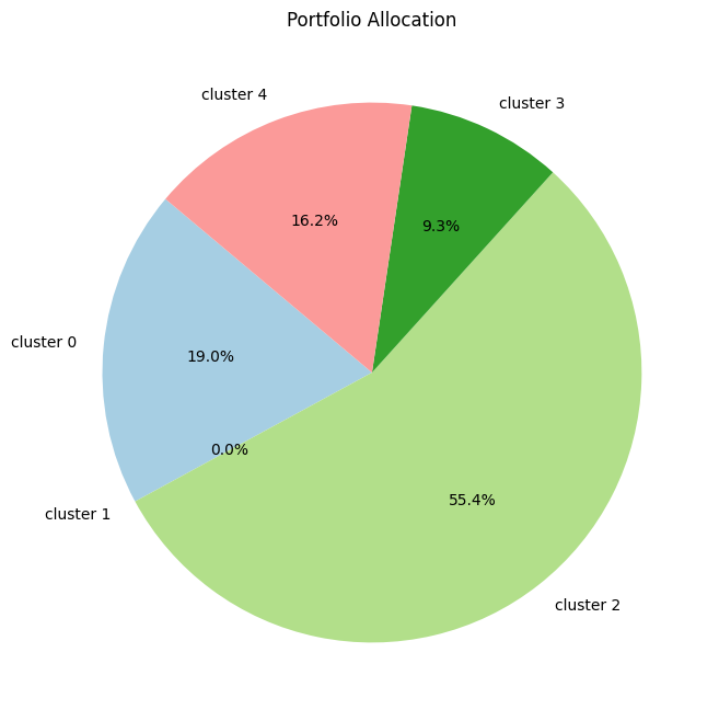
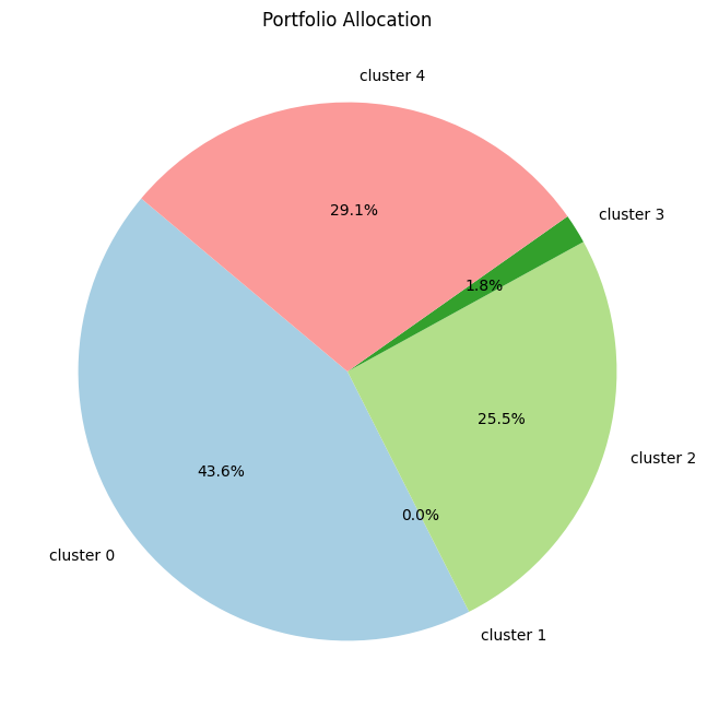
Firstly, an equiponderated (equal-weighted) strategy will be used within each cluster. This approach simplifies the investment process by equally distributing capital across all assets within a cluster, under the assumption that each asset contributes equally to the risk-return profile of the cluster. This method will serve as a baseline to assess the effectiveness of clustering in portfolio diversification without the influence of optimization techniques.
Maximizing Sharpe Ratio Within Clusters
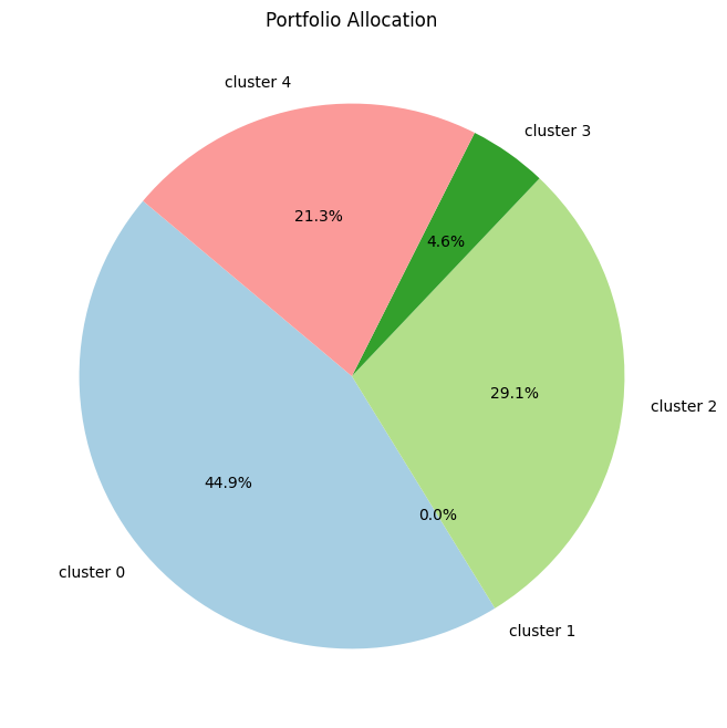
Subsequently, the course will explore a more refined optimization strategy within each cluster by maximizing the Sharpe ratio. The Sharpe ratio is a measure of risk-adjusted return, and maximizing it within each cluster aims to find the most efficient combination of assets that provides the best return for a given level of risk. This involves solving an optimization problem similar to the Markowitz optimization, but with the focus narrowed down to assets within each cluster.
Course Goals for Clustering Application
By employing these two approaches, the course intends to:
Evaluate Clustering Effectiveness: Determine whether clustering can provide a more efficient asset allocation by reducing intra-portfolio correlation and thus potentially lowering overall portfolio risk.
Compare Allocation Strategies: Assess the performance difference between a simple equal-weighted allocation and a more sophisticated optimization within clusters, to identify which method may be more advantageous in the context of clustered assets.
Practical Application: Examine the practical implications of implementing these strategies, considering transaction costs, rebalancing frequencies, and the manageability of the strategies in a real-world setting.
from sklearn.cluster import AffinityPropagation, AgglomerativeClustering, Birch, DBSCAN, HDBSCAN, KMeans, BisectingKMeans, MeanShift, SpectralClustering, SpectralBiclustering
from sklearn.mixture import GaussianMixture
n_cluster = 5
prices = get_prices(data_train, final_assets)
returns = compute_returns(prices)
clustering_model = SpectralClustering(
n_clusters=n_cluster,
random_state=42,
)
clusters = clustering_model.fit_predict(returns.T)Equiponderated within clusters
# Initialize an empty list to store aggregated returns for each cluster
clustered_returns = []
intra_clusters_weights, intra_clusters_indice_equivalent = [], []
# Loop through each cluster
for i in range(max(clusters) + 1):
    # Find indices of stocks belonging to the current cluster
    cluster_indices = np.where(clusters == i)[0]

    # Check if the cluster is not empty
    if len(cluster_indices) > 0:
        # Calculate the mean return of stocks in the cluster
        intra_cluster_weights = np.ones(len(cluster_indices)) / len(cluster_indices)
        intra_clusters_weights.append(intra_cluster_weights)
        intra_clusters_indice_equivalent.append(cluster_indices)
        cluster_returns = (returns.iloc[:, cluster_indices] * intra_cluster_weights).sum(axis=1)
        clustered_returns.append(cluster_returns)
    else:
        # If the cluster is empty, append a series of zeros
        clustered_returns.append(pd.Series(np.zeros(len(returns)), index=df_returns.index))

# Convert the list of aggregated returns to a DataFrame
clustered_returns_df = pd.concat(clustered_returns, axis=1)
print(clustered_returns_df)
0 1 2 3 4
group
2019-12-13 16:00:00 0.000510 0.010792 0.001602 -0.001919 0.000154
2019-12-13 17:00:00 -0.002998 -0.007884 -0.003858 0.003452 0.000606
2019-12-13 18:00:00 -0.002406 -0.007289 -0.002805 0.002042 -0.004247
2019-12-13 19:00:00 -0.001250 0.015096 0.004723 0.003393 0.000750
2019-12-13 20:00:00 -0.001825 -0.003940 0.000157 -0.001947 0.001425
... ... ... ... ... ...
2021-06-23 16:00:00 0.012061 0.019515 0.013206 0.011816 0.013534
2021-06-23 17:00:00 -0.007332 -0.010834 -0.005624 -0.002292 -0.010083
2021-06-23 18:00:00 -0.020280 -0.022765 -0.024415 -0.029693 -0.025710
2021-06-23 19:00:00 -0.016569 -0.014792 -0.016333 -0.013520 -0.020060
2021-06-23 20:00:00 0.015444 0.017494 0.010074 0.005466 0.012936
[13397 rows x 5 columns]Compute efficient frontier and select an optimal allocation
# Compute mean returns and covariance matrix for each cluster
mu_clusters = clustered_returns_df.mean()
sigma_clusters = clustered_returns_df.cov()

plot_optimized_efficient_frontier(mu_clusters, sigma_clusters, show=False)
plot_monte_carlo_only_efficient_frontier(mu_clusters, sigma_clusters, show=False)
plt.show()

optimization_result = optimize_portfolio(mu_clusters, sigma_clusters, maximum_volatility)
if optimization_result.success:
    optimal_cluster_weights = optimization_result.x
    # Create the pie chart
    plt.figure(figsize=(8, 8))
    plt.pie(optimal_cluster_weights, labels=[f'cluster {i}' for i in range(n_cluster)], autopct='%1.1f%%', startangle=140, colors=plt.cm.Paired.colors)

    # Adding title
    plt.title('Portfolio Allocation')

    # Show the plot
    plt.show()
else:
    print("Did not converge")


print('\n'*3)
Get back from cluster weights to asset weight
optimal_asset_weights = []
for i in range(prices.shape[1]):
    cluster_index = clusters[i]
    intra_cluster_weight = intra_clusters_weights[cluster_index][np.where(intra_clusters_indice_equivalent[cluster_index]==i)[0][0]]
    optimal_asset_weights.append(optimal_cluster_weights[cluster_index] * intra_cluster_weight)
optimal_asset_weights = np.array(optimal_asset_weights)
plt.figure(figsize=(8, 8))
plt.pie(optimal_asset_weights, labels=final_assets, autopct='%1.1f%%', startangle=140, colors=plt.cm.Paired.colors)

# Adding title
plt.title('Portfolio Allocation')

# Show the plot
plt.show()
Backtesting the method
backtest(optimal_asset_weights, final_assets, method='continuous')On train using continuous reponderation:
optimized_porfolio_value has an expected return of 2.6200146302148486 for a risk of 1.1000409772296078
equiponderated_porfolio_value has an expected return of 2.571030019068987 for a risk of 1.1033719694757085
btc_only_porfolio_value has an expected return of 1.3450136751201247 for a risk of 0.8411451768924758
On test using continuous reponderation:
optimized_porfolio_value has an expected return of 0.23315697286958578 for a risk of 0.8582715788281714
equiponderated_porfolio_value has an expected return of 0.09317371980719207 for a risk of 0.872321680813382
btc_only_porfolio_value has an expected return of -0.24874776856528497 for a risk of 0.6432098891396297Maximising Sharpe within clusters
def optimize_portfolio_sharpe(expected_returns, cov_matrix):
    num_assets = len(expected_returns)
    args = (expected_returns, cov_matrix)
    constraints = ({'type': 'eq', 'fun': lambda x: np.sum(x) - 1})
    bounds = tuple((0, 1) for asset in range(num_assets))

    def objective_function(weights, expected_returns, cov_matrix):
        return -portfolio_annualized_expected_return(weights, expected_returns) / portfolio_annualized_risk(weights, cov_matrix)

    result = minimize(objective_function, num_assets*[1./num_assets,], args=args, method='SLSQP', bounds=bounds, constraints=constraints)
    return result

prices = get_prices(data_train, final_assets)
returns = compute_returns(prices)
# Initialize an empty list to store aggregated returns for each cluster
clustered_returns = []
intra_clusters_weights, intra_clusters_indice_equivalent = [], []
# Loop through each cluster
for i in range(max(clusters) + 1):
    # Find indices of stocks belonging to the current cluster
    cluster_indices = np.where(clusters == i)[0]

    # Check if the cluster is not empty
    if len(cluster_indices) > 0:
        # Calculate the mean return of stocks in the cluster

        prices_cluster = prices.iloc[:, cluster_indices]
        returns_cluster = compute_returns(prices_cluster)
        mu_cluster = returns_cluster.mean()
        sigmas_cluster = returns_cluster.cov()
        optimization_result = optimize_portfolio_sharpe(mu_cluster, sigmas_cluster)
        if optimization_result.success:
            intra_cluster_weights = optimization_result.x
            print('Optimization succeed, intra_cluster_weights=', intra_cluster_weights)
        else:
            print('Optimization did not converge for cluster {} - using equiponderation instead')
            intra_cluster_weights = np.ones(len(cluster_indices)) / len(cluster_indices)

        intra_clusters_weights.append(intra_cluster_weights)
        intra_clusters_indice_equivalent.append(cluster_indices)
        cluster_returns = (returns.iloc[:, cluster_indices] * intra_cluster_weights).sum(axis=1)
        clustered_returns.append(cluster_returns)
    else:
        # If the cluster is empty, append a series of zeros
        clustered_returns.append(pd.Series(np.zeros(len(returns)), index=df_returns.index))

# Convert the list of aggregated returns to a DataFrame
clustered_returns_df = pd.concat(clustered_returns, axis=1)
Optimization succeed, intra_cluster_weights= [4.16341678e-16 3.72641715e-01 1.56063425e-17 0.00000000e+00
0.00000000e+00 0.00000000e+00 1.29074771e-16 0.00000000e+00
2.67677130e-01 3.57266025e-16 0.00000000e+00 0.00000000e+00
0.00000000e+00 1.35855622e-16 2.10684032e-16 3.59681155e-01
1.55340471e-16 0.00000000e+00 0.00000000e+00 4.73854450e-16
0.00000000e+00 2.02571278e-16 0.00000000e+00 1.05887380e-16
8.66126609e-16]
Optimization succeed, intra_cluster_weights= [0.40630611 0.59369389]
Optimization succeed, intra_cluster_weights= [0.00000000e+00 9.85294704e-16 6.36700128e-02 2.01523641e-01
0.00000000e+00 0.00000000e+00 3.85078857e-03 7.82494271e-02
7.22489349e-02 0.00000000e+00 4.19781711e-03 4.81605601e-02
6.62861762e-03 1.67554108e-02 3.22977781e-16 0.00000000e+00
4.81483991e-02 4.36996624e-16 2.38667296e-01 3.67593109e-17
1.08455698e-01 6.02486376e-16 1.09443397e-01]
Optimization succeed, intra_cluster_weights= [0.54157708 0.45842292]
Optimization succeed, intra_cluster_weights= [8.96372635e-02 2.80098111e-16 2.30010177e-01 1.58703016e-01
4.33777520e-18 6.75088384e-02 1.49667252e-16 3.54498291e-17
2.61802336e-16 6.75436045e-17 4.46435474e-17 7.32146748e-16
5.40789232e-02 6.22603222e-17 9.69209852e-02 5.72043462e-16
3.03140797e-01 7.32832895e-17]Compute efficient frontier and select an optimal allocation
# Compute mean returns and covariance matrix for each cluster
mu_clusters = clustered_returns_df.mean()
sigma_clusters = clustered_returns_df.cov()

plot_optimized_efficient_frontier(mu_clusters, sigma_clusters, show=False)
plot_monte_carlo_only_efficient_frontier(mu_clusters, sigma_clusters, show=False)
plt.show()

optimization_result = optimize_portfolio(mu_clusters, sigma_clusters, maximum_volatility)
if optimization_result.success:
    optimal_cluster_weights = optimization_result.x
    # Create the pie chart
    plt.figure(figsize=(8, 8))
    plt.pie(optimal_cluster_weights, labels=[f'cluster {i}' for i in range(n_cluster)], autopct='%1.1f%%', startangle=140, colors=plt.cm.Paired.colors)

    # Adding title
    plt.title('Portfolio Allocation')

    # Show the plot
    plt.show()
else:
    print("Did not converge")


print('\n'*3)
optimal_asset_weights = []
for i in range(prices.shape[1]):
    cluster_index = clusters[i]
    intra_cluster_weight = intra_clusters_weights[cluster_index][np.where(intra_clusters_indice_equivalent[cluster_index]==i)[0][0]]
    optimal_asset_weights.append(optimal_cluster_weights[cluster_index] * intra_cluster_weight)
optimal_asset_weights = np.array(optimal_asset_weights)
plt.figure(figsize=(8, 8))
plt.pie(optimal_asset_weights, labels=final_assets, autopct='%1.1f%%', startangle=140, colors=plt.cm.Paired.colors)

# Adding title
plt.title('Portfolio Allocation')

# Show the plot
plt.show()
Backtesting the method
backtest(optimal_asset_weights, final_assets, method='continuous')On train using continuous reponderation:
optimized_porfolio_value has an expected return of 3.8037353911260974 for a risk of 1.100040444337943
equiponderated_porfolio_value has an expected return of 2.571030019068987 for a risk of 1.1033719694757085
btc_only_porfolio_value has an expected return of 1.3450136751201247 for a risk of 0.8411451768924758
On test using continuous reponderation:
optimized_porfolio_value has an expected return of -0.1357167801817761 for a risk of 0.8713191363042782
equiponderated_porfolio_value has an expected return of 0.09317371980719207 for a risk of 0.872321680813382
btc_only_porfolio_value has an expected return of -0.24874776856528497 for a risk of 0.64320988913962971. Diversification through Equally Weighted Clusters
The approach of using clustering to form groups of assets and then applying equal weighting within those clusters has demonstrated promising results. By dispersifying investments across different clusters, the risk associated with over-concentration in any single asset or market segment is mitigated. The more even distribution of capital leads to a portfolio that benefits from the unique characteristics of each cluster. In the test set, this method has shown to contain risk effectively while delivering superior returns compared to previous methods. The improved performance in the test set underscores the value of diversification, especially in markets like cryptocurrencies, where the risk of rapid and significant price movements is high.
2. Limitations of Excessive Optimization within Clusters
On the other hand, adding another layer of optimization within clusters by maximizing the Sharpe ratio appears to have counterintuitive effects. Although theoretically, this should refine the portfolio further by adjusting weights to the risk-return profile of individual assets within each cluster, it can inadvertently lead to a concentration of weights. This concentration may negate some of the diversification benefits offered by clustering, resulting in a less diversified portfolio. In the example provided, this excessive focus on optimization within clusters led to underperformance, suggesting that there is a delicate balance between beneficial asset allocation and over-optimization that might expose the portfolio to unanticipated risks.
Conclusions and Course Trajectory
These findings suggest that while clustering is a powerful tool for enhancing portfolio diversification, the way in which assets are weighted within clusters is pivotal. A simple equal-weighted approach within clusters seems to strike an effective balance between diversification and performance. It supports the idea that sometimes, a less complex model can be more resilient and successful, particularly in unpredictable markets.
The results also highlight the potential drawbacks of over-optimization. In striving for perfection in asset weightings based on historical performance, one may inadvertently introduce biases or overfit to past data, which do not necessarily predict future market conditions.
Testing other rules :
Using example before, you can try different options, from choosing other clusterisation methods, modifying number of clusters, selecting weights within clusters differently etc… For example bellow, you can give set the maximum volatility target of the cluster to be equal to the equally weighted one plus or minus a volatility budget ! With all what’s above you have more than enough to play with
for vol_budget in [-0.1, -0.05, -0.02, 0, 0.02, 0.05, 0.1]:

    print(f'for a volatility budget within cluster compared to equiponderated of {vol_budget}')

    prices = get_prices(data_train, final_assets)
    returns = compute_returns(prices)
    # Initialize an empty list to store aggregated returns for each cluster
    clustered_returns = []
    intra_clusters_weights, intra_clusters_indice_equivalent = [], []
    # Loop through each cluster
    for i in range(max(clusters) + 1):
        # Find indices of stocks belonging to the current cluster
        cluster_indices = np.where(clusters == i)[0]

        # Check if the cluster is not empty
        if len(cluster_indices) > 0:
            # Calculate the mean return of stocks in the cluster

            prices_cluster = prices.iloc[:, cluster_indices]
            returns_cluster = compute_returns(prices_cluster)
            mu_cluster = returns_cluster.mean()
            sigmas_cluster = returns_cluster.cov()
            optimization_result = optimize_portfolio(mu_cluster, sigmas_cluster, returns_cluster.mean(axis=1).std() * np.sqrt(365*24) * (1.1+vol_budget))
            if optimization_result.success:
                intra_cluster_weights = optimization_result.x
                print('Optimization succeed, intra_cluster_weights=', intra_cluster_weights)
            else:
                print('Optimization did not converge for cluster {} - using equiponderation instead')
                intra_cluster_weights = np.ones(len(cluster_indices)) / len(cluster_indices)

            intra_clusters_weights.append(intra_cluster_weights)
            intra_clusters_indice_equivalent.append(cluster_indices)
            cluster_returns = (returns.iloc[:, cluster_indices] * intra_cluster_weights).sum(axis=1)
            clustered_returns.append(cluster_returns)
        else:
            # If the cluster is empty, append a series of zeros
            clustered_returns.append(pd.Series(np.zeros(len(returns)), index=df_returns.index))

    # Convert the list of aggregated returns to a DataFrame
    clustered_returns_df = pd.concat(clustered_returns, axis=1)

    # Compute mean returns and covariance matrix for each cluster
    mu_clusters = clustered_returns_df.mean()
    sigma_clusters = clustered_returns_df.cov()

    plot_optimized_efficient_frontier(mu_clusters, sigma_clusters, show=False)
    plot_monte_carlo_only_efficient_frontier(mu_clusters, sigma_clusters, show=False)
    plt.show()

    optimization_result = optimize_portfolio(mu_clusters, sigma_clusters, maximum_volatility)
    if optimization_result.success:
        optimal_cluster_weights = optimization_result.x
        # Create the pie chart
        plt.figure(figsize=(8, 8))
        plt.pie(optimal_cluster_weights, labels=[f'cluster {i}' for i in range(n_cluster)], autopct='%1.1f%%', startangle=140, colors=plt.cm.Paired.colors)

        # Adding title
        plt.title('Portfolio Allocation')

        # Show the plot
        plt.show()
    else:
        print("Did not converge")


    print('\n'*3)
    optimal_asset_weights = []
    for i in range(prices.shape[1]):
        cluster_index = clusters[i]
        intra_cluster_weight = intra_clusters_weights[cluster_index][np.where(intra_clusters_indice_equivalent[cluster_index]==i)[0][0]]
        optimal_asset_weights.append(optimal_cluster_weights[cluster_index] * intra_cluster_weight)
    optimal_asset_weights = np.array(optimal_asset_weights)
    plt.figure(figsize=(8, 8))
    plt.pie(optimal_asset_weights, labels=final_assets, autopct='%1.1f%%', startangle=140, colors=plt.cm.Paired.colors)

    # Adding title
    plt.title('Portfolio Allocation')

    # Show the plot
    plt.show()


    backtest(optimal_asset_weights, final_assets, method='continuous')

    print('\n'*4)
for a volatility budget within cluster compared to equiponderated of -0.1
Optimization succeed, intra_cluster_weights= [2.54382263e-02 2.58498645e-01 0.00000000e+00 0.00000000e+00
1.61733360e-15 0.00000000e+00 0.00000000e+00 0.00000000e+00
2.48974847e-01 0.00000000e+00 0.00000000e+00 0.00000000e+00
0.00000000e+00 3.49073289e-16 0.00000000e+00 2.61704766e-01
3.59343563e-16 3.62083292e-16 1.40749644e-15 0.00000000e+00
2.62604608e-15 1.02780164e-15 2.05383515e-01 0.00000000e+00
0.00000000e+00]
Optimization succeed, intra_cluster_weights= [0.46984352 0.53015648]
Optimization succeed, intra_cluster_weights= [5.58449135e-16 0.00000000e+00 8.19396144e-02 1.10026782e-01
8.12685993e-17 1.31669934e-16 3.99402771e-02 9.45435688e-02
3.04904613e-02 6.68352315e-16 4.56835953e-02 3.39414874e-02
7.72588767e-02 3.25521002e-02 4.98313995e-02 1.51079621e-02
6.87895449e-02 3.17196858e-16 9.69036318e-02 4.06025305e-02
5.64218394e-02 1.88511033e-03 1.24081218e-01]
Optimization succeed, intra_cluster_weights= [0.5 0.5]
Optimization succeed, intra_cluster_weights= [9.29868998e-02 0.00000000e+00 1.29531108e-01 1.40927040e-01
6.38232427e-02 2.07918025e-02 0.00000000e+00 8.07074528e-02
0.00000000e+00 2.78931719e-02 0.00000000e+00 0.00000000e+00
3.28381236e-02 4.37712111e-16 2.17546800e-01 1.87719339e-02
1.67093861e-01 7.08856400e-03]
On train using continuous reponderation:
optimized_porfolio_value has an expected return of 3.605486250587928 for a risk of 1.1000408810602653
equiponderated_porfolio_value has an expected return of 2.571030019068987 for a risk of 1.1033719694757085
btc_only_porfolio_value has an expected return of 1.3450136751201247 for a risk of 0.8411451768924758
On test using continuous reponderation:
optimized_porfolio_value has an expected return of -0.2093157303510894 for a risk of 0.8942899519600324
equiponderated_porfolio_value has an expected return of 0.09317371980719207 for a risk of 0.872321680813382
btc_only_porfolio_value has an expected return of -0.24874776856528497 for a risk of 0.6432098891396297
for a volatility budget within cluster compared to equiponderated of -0.05
Optimization succeed, intra_cluster_weights= [5.93474964e-15 3.17505540e-01 3.22928109e-15 1.28603365e-15
5.07262649e-15 3.84376592e-15 2.95423570e-15 6.64207742e-16
2.61900581e-01 0.00000000e+00 2.86442266e-15 1.00976921e-15
2.48969259e-16 0.00000000e+00 2.43850858e-15 3.11525817e-01
1.02141076e-16 2.23850608e-15 0.00000000e+00 2.05855272e-15
0.00000000e+00 0.00000000e+00 1.09068062e-01 2.69686967e-15
2.46612802e-15]
Optimization succeed, intra_cluster_weights= [0.16631208 0.83368792]
Optimization succeed, intra_cluster_weights= [0. 0. 0.07600087 0.16633709 0. 0.
0.02294429 0.08879252 0.05586648 0. 0.025294 0.04646625
0.04121012 0.02645711 0. 0. 0.06130096 0.
0.18086966 0. 0.0892339 0. 0.11922675]
Optimization succeed, intra_cluster_weights= [0.41206396 0.58793604]
Optimization succeed, intra_cluster_weights= [9.74850397e-02 0.00000000e+00 1.99581890e-01 1.65664181e-01
1.43361927e-02 5.49820290e-02 6.65374873e-16 1.39468210e-16
0.00000000e+00 0.00000000e+00 9.18935033e-16 6.23023226e-16
5.51282083e-02 5.23873784e-16 1.63653745e-01 1.13447358e-15
2.49168714e-01 0.00000000e+00]
On train using continuous reponderation:
optimized_porfolio_value has an expected return of 3.790927125465613 for a risk of 1.100040964920101
equiponderated_porfolio_value has an expected return of 2.571030019068987 for a risk of 1.1033719694757085
btc_only_porfolio_value has an expected return of 1.3450136751201247 for a risk of 0.8411451768924758
On test using continuous reponderation:
optimized_porfolio_value has an expected return of -0.145692461412965 for a risk of 0.8845218213316236
equiponderated_porfolio_value has an expected return of 0.09317371980719207 for a risk of 0.872321680813382
btc_only_porfolio_value has an expected return of -0.24874776856528497 for a risk of 0.6432098891396297
for a volatility budget within cluster compared to equiponderated of -0.02
Optimization succeed, intra_cluster_weights= [1.35643831e-15 3.51912328e-01 0.00000000e+00 0.00000000e+00
1.60772548e-15 3.31385450e-15 1.99215503e-15 0.00000000e+00
2.66949976e-01 0.00000000e+00 1.34336687e-15 0.00000000e+00
8.71946874e-16 0.00000000e+00 1.40747773e-15 3.40653615e-01
1.01685577e-16 1.64620805e-15 0.00000000e+00 1.47850464e-15
0.00000000e+00 0.00000000e+00 4.04840805e-02 2.13293026e-15
1.50606510e-15]
Optimization succeed, intra_cluster_weights= [0.07914572 0.92085428]
Optimization succeed, intra_cluster_weights= [0. 0. 0.06667508 0.19283431 0. 0.
0.00861775 0.08084719 0.06819132 0. 0.00949222 0.04777252
0.01509857 0.01912904 0. 0. 0.05154913 0.
0.2242508 0. 0.10370019 0. 0.11184187]
Optimization succeed, intra_cluster_weights= [0.36883408 0.63116592]
Optimization succeed, intra_cluster_weights= [9.04171921e-02 2.34933397e-15 2.27665246e-01 1.59564894e-01
0.00000000e+00 6.65699401e-02 1.12528666e-15 1.42343887e-16
2.92988696e-16 5.04526705e-17 1.20337971e-16 1.89010320e-16
5.43354460e-02 0.00000000e+00 1.02653671e-01 0.00000000e+00
2.98793611e-01 0.00000000e+00]
On train using continuous reponderation:
optimized_porfolio_value has an expected return of 3.8142362297455037 for a risk of 1.1000405407473406
equiponderated_porfolio_value has an expected return of 2.571030019068987 for a risk of 1.1033719694757085
btc_only_porfolio_value has an expected return of 1.3450136751201247 for a risk of 0.8411451768924758
On test using continuous reponderation:
optimized_porfolio_value has an expected return of -0.1336961707119556 for a risk of 0.8746162158674432
equiponderated_porfolio_value has an expected return of 0.09317371980719207 for a risk of 0.872321680813382
btc_only_porfolio_value has an expected return of -0.24874776856528497 for a risk of 0.6432098891396297
for a volatility budget within cluster compared to equiponderated of 0
Optimization succeed, intra_cluster_weights= [0.00000000e+00 3.72685177e-01 0.00000000e+00 0.00000000e+00
0.00000000e+00 0.00000000e+00 0.00000000e+00 0.00000000e+00
2.67988244e-01 0.00000000e+00 0.00000000e+00 0.00000000e+00
0.00000000e+00 1.42705270e-15 0.00000000e+00 3.59326579e-01
0.00000000e+00 0.00000000e+00 8.32345910e-16 0.00000000e+00
2.87693732e-15 8.48163901e-16 0.00000000e+00 0.00000000e+00
0.00000000e+00]
Optimization succeed, intra_cluster_weights= [0.02913959 0.97086041]
Optimization succeed, intra_cluster_weights= [3.53879693e-15 9.34846362e-15 6.14566414e-02 2.07643399e-01
0.00000000e+00 2.88335292e-15 6.33412415e-04 7.64475154e-02
7.50515558e-02 5.53070160e-15 6.81741856e-04 4.85088311e-02
5.16355971e-04 1.50540609e-02 6.32528823e-15 1.52654551e-15
4.60730094e-02 5.17085151e-15 2.48452618e-01 3.04516995e-15
1.11732261e-01 6.32558163e-15 1.07748598e-01]
Optimization succeed, intra_cluster_weights= [0.34231845 0.65768155]
Optimization succeed, intra_cluster_weights= [8.53123910e-02 2.74180415e-15 2.42765905e-01 1.54145436e-01
7.64979172e-16 7.25279557e-02 1.10581761e-15 4.70641152e-16
1.69244213e-15 1.16243244e-15 1.98297105e-15 2.36618484e-15
5.27062096e-02 4.34520279e-16 6.51630248e-02 2.56601940e-15
3.27379078e-01 5.52469617e-16]
On train using continuous reponderation:
optimized_porfolio_value has an expected return of 3.7934023531589163 for a risk of 1.10004026277759
equiponderated_porfolio_value has an expected return of 2.571030019068987 for a risk of 1.1033719694757085
btc_only_porfolio_value has an expected return of 1.3450136751201247 for a risk of 0.8411451768924758
On test using continuous reponderation:
optimized_porfolio_value has an expected return of -0.12128328860898158 for a risk of 0.8665326522617827
equiponderated_porfolio_value has an expected return of 0.09317371980719207 for a risk of 0.872321680813382
btc_only_porfolio_value has an expected return of -0.24874776856528497 for a risk of 0.6432098891396297
for a volatility budget within cluster compared to equiponderated of 0.02
Optimization succeed, intra_cluster_weights= [1.35074328e-15 3.80893112e-01 2.16788312e-17 0.00000000e+00
1.49316962e-15 0.00000000e+00 3.64832122e-16 4.49307345e-16
2.32760672e-01 2.00059341e-16 0.00000000e+00 0.00000000e+00
1.69484237e-16 0.00000000e+00 7.85905124e-16 3.86346216e-01
1.11937636e-15 0.00000000e+00 7.72258156e-16 9.29769937e-16
6.29386023e-16 1.14995748e-16 0.00000000e+00 0.00000000e+00
1.70789254e-16]
Optimization succeed, intra_cluster_weights= [0. 1.]
Optimization succeed, intra_cluster_weights= [7.94255548e-15 8.57361259e-15 5.01574185e-02 2.22184731e-01
5.95400126e-16 5.47923674e-15 3.96836694e-16 6.65062268e-02
8.17664211e-02 1.36385456e-14 2.31566062e-15 4.50380397e-02
2.98706890e-15 6.19742127e-03 1.16863898e-14 3.48202916e-15
3.47047849e-02 9.71471820e-15 2.75394962e-01 5.28291145e-15
1.18980580e-01 1.20492174e-14 9.90694147e-02]
Optimization succeed, intra_cluster_weights= [0.31719603 0.68280397]
Optimization succeed, intra_cluster_weights= [8.07475028e-02 1.19997531e-14 2.56226229e-01 1.49318887e-01
1.41935278e-15 7.78297056e-02 5.47245287e-15 3.20562668e-15
6.26149455e-15 6.63545621e-15 5.11510322e-15 1.04007311e-14
5.12618217e-02 3.47413613e-15 3.17925682e-02 1.04024624e-14
3.52823286e-01 1.49232298e-15]
Did not converge
On train using continuous reponderation:
optimized_porfolio_value has an expected return of 3.854842353198852 for a risk of 1.1095879959629442
equiponderated_porfolio_value has an expected return of 2.571030019068987 for a risk of 1.1033719694757085
btc_only_porfolio_value has an expected return of 1.3450136751201247 for a risk of 0.8411451768924758
On test using continuous reponderation:
optimized_porfolio_value has an expected return of -0.12478129130353557 for a risk of 0.8740310124849314
equiponderated_porfolio_value has an expected return of 0.09317371980719207 for a risk of 0.872321680813382
btc_only_porfolio_value has an expected return of -0.24874776856528497 for a risk of 0.6432098891396297
for a volatility budget within cluster compared to equiponderated of 0.05
Optimization succeed, intra_cluster_weights= [0.00000000e+00 3.91961427e-01 0.00000000e+00 0.00000000e+00
0.00000000e+00 0.00000000e+00 0.00000000e+00 3.33324972e-16
1.85244250e-01 0.00000000e+00 0.00000000e+00 0.00000000e+00
0.00000000e+00 9.24554064e-16 0.00000000e+00 4.22794323e-01
0.00000000e+00 0.00000000e+00 0.00000000e+00 0.00000000e+00
7.97627596e-16 1.12510926e-15 0.00000000e+00 0.00000000e+00
0.00000000e+00]
Optimization succeed, intra_cluster_weights= [0. 1.]
Optimization succeed, intra_cluster_weights= [9.63936162e-16 1.74633504e-15 3.38389705e-02 2.41337594e-01
0.00000000e+00 0.00000000e+00 3.13312187e-16 5.18461389e-02
9.00094829e-02 2.21008781e-15 1.06622464e-16 3.93036826e-02
3.14217270e-16 4.43544042e-16 7.44079745e-16 0.00000000e+00
1.76697472e-02 1.53297582e-16 3.11289077e-01 9.19944861e-16
1.28344220e-01 1.35045637e-15 8.63610858e-02]
Optimization succeed, intra_cluster_weights= [0.28158 0.71842]
Optimization succeed, intra_cluster_weights= [6.95960511e-02 3.69224711e-15 2.73511605e-01 1.33804517e-01
0.00000000e+00 8.39890929e-02 8.53912887e-16 6.19719944e-16
3.99403987e-16 8.09600020e-16 0.00000000e+00 1.21183225e-15
4.37406839e-02 0.00000000e+00 3.46447487e-16 8.55203427e-16
3.95358050e-01 0.00000000e+00]
Did not converge
On train using continuous reponderation:
optimized_porfolio_value has an expected return of 3.936954827163496 for a risk of 1.1234058575131143
equiponderated_porfolio_value has an expected return of 2.571030019068987 for a risk of 1.1033719694757085
btc_only_porfolio_value has an expected return of 1.3450136751201247 for a risk of 0.8411451768924758
On test using continuous reponderation:
optimized_porfolio_value has an expected return of -0.1300400607391719 for a risk of 0.8838683381483989
equiponderated_porfolio_value has an expected return of 0.09317371980719207 for a risk of 0.872321680813382
btc_only_porfolio_value has an expected return of -0.24874776856528497 for a risk of 0.6432098891396297
for a volatility budget within cluster compared to equiponderated of 0.1
Optimization succeed, intra_cluster_weights= [0.00000000e+00 4.08295613e-01 0.00000000e+00 0.00000000e+00
0.00000000e+00 0.00000000e+00 0.00000000e+00 0.00000000e+00
1.15221210e-01 0.00000000e+00 0.00000000e+00 4.78907552e-17
0.00000000e+00 6.99555893e-16 0.00000000e+00 4.76483177e-01
3.70717639e-16 0.00000000e+00 9.23634606e-16 0.00000000e+00
1.36479388e-15 6.35036830e-16 0.00000000e+00 0.00000000e+00
0.00000000e+00]
Optimization succeed, intra_cluster_weights= [0. 1.]
Optimization succeed, intra_cluster_weights= [2.90464713e-16 0.00000000e+00 6.36173555e-03 2.67973871e-01
0.00000000e+00 0.00000000e+00 2.05152594e-16 2.70524358e-02
1.00782773e-01 0.00000000e+00 0.00000000e+00 2.80802982e-02
0.00000000e+00 7.88257135e-18 0.00000000e+00 0.00000000e+00
1.49229798e-16 0.00000000e+00 3.63851874e-01 3.80425010e-16
1.40858704e-01 0.00000000e+00 6.50383088e-02]
Optimization succeed, intra_cluster_weights= [0.22637548 0.77362452]
Optimization succeed, intra_cluster_weights= [0.03793037 0. 0.29417604 0.08348462 0. 0.08906395
0. 0. 0. 0. 0. 0.
0.01545689 0. 0. 0. 0.47988813 0. ]
Did not converge
On train using continuous reponderation:
optimized_porfolio_value has an expected return of 4.054156484432186 for a risk of 1.1451497547686114
equiponderated_porfolio_value has an expected return of 2.571030019068987 for a risk of 1.1033719694757085
btc_only_porfolio_value has an expected return of 1.3450136751201247 for a risk of 0.8411451768924758
On test using continuous reponderation:
optimized_porfolio_value has an expected return of -0.14557169301657574 for a risk of 0.8971616013141652
equiponderated_porfolio_value has an expected return of 0.09317371980719207 for a risk of 0.872321680813382
btc_only_porfolio_value has an expected return of -0.24874776856528497 for a risk of 0.6432098891396297
