In this course, we explore how the expressivity of deep learning can simplify the representation and resolution of complex decision problems—in our case, the problem of VWAP (Volume-Weighted Average Price) order execution.
Telecharger le notebook
Telecharger les donnes de notionnel
Telecharger les donnes de volume
1. Introduction to Order Execution and Order Books
Before diving into deep learning, we begin by understanding the fundamentals:
What is an Order?
An order is a request to buy or sell a financial asset. In trading, orders come in different types (e.g., market orders, limit orders) that dictate execution conditions.
Order Book:
The order book is a real-time record of all outstanding buy and sell orders for a given asset. It reflects the market’s supply and demand, and understanding it is crucial for grasping how trades are executed.
2. Market Impact
When executing orders, especially large ones, traders must consider the market impact—the effect that the order has on the asset’s price. There are two main components:
Temporary Market Impact: Short-term price movements caused by the execution of the order.
Permanent Market Impact: Lasting changes in price due to the information conveyed by the trade.
The goal is to minimize these impacts so that the execution price remains as close as possible to the prevailing market price.
3. Splitting Orders Over Time
To reduce market impact, large orders are typically divided into smaller portions and executed over time. This process involves:
Breaking down the order:
Executing a fraction of the total order at regular intervals helps to mitigate the adverse effects on the market.
Balancing challenge:
The challenge lies in determining how much volume to execute at each interval to minimize the deviation from a fair benchmark.
4. Benchmarking with VWAP
The Volume-Weighted Average Price (VWAP) serves as an ideal benchmark for order execution. VWAP is defined as:
where ( p_i ) is the price of the ( i )-th trade and ( v_i ) is its volume. The ideal scenario is that the sum of the overperformance (the difference between the executed price and the market VWAP) is zero.
Why VWAP?
VWAP provides a neutral reference that reflects the average price traded over a period, making it a fair standard for evaluating execution performance.
5. Order Allocation Over Time
Our primary objective is to allocate the total order across multiple time intervals such that:
The execution price (i.e., the weighted average price at which our trades are executed) aligns closely with the market VWAP.
The volume allocation in each time interval is optimally determined to minimize both price deviation and market impact.
This problem naturally decomposes into two sub-problems: - Price Deviation Minimization: Ensuring that the price paid in each interval is as close as possible to the market price. - Volume Allocation Optimization: Adjusting the fraction of the order executed in each interval to mirror the market’s volume profile effectively.
TP Part 1: Data Exploration and VWAP Calculation
In this exercise, you will work with BTC data to get hands-on experience with the basic computations needed for VWAP-based order execution. Follow these steps:
Objectives:
Load the Data:
Load the notional and volume data for BTC using pd.read_parquet. Hint: Use the provided variables below.
Compute the VWAP:
Calculate the VWAP at each time point as the ratio of notional to volume. If there are missing values (NaNs), apply a forward fill.
Compute Returns:
Compute the percentage returns over time using the computed VWAP as the price.
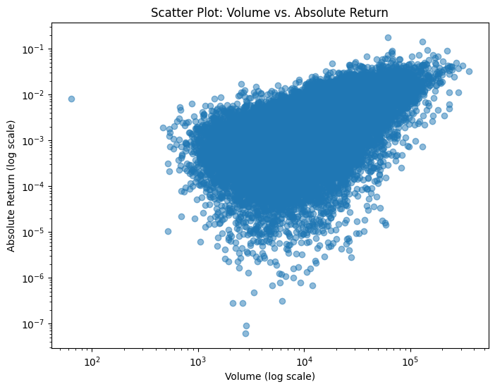
Scatter Plot:
Create a scatter plot of volume versus absolute returns, using logarithmic scales on both axes.
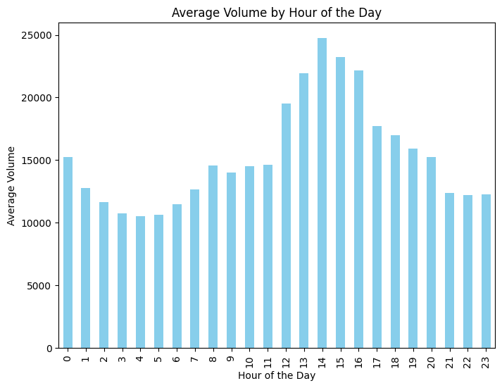
Average Volume by Hour:
Create a new column for the hour extracted from the datetime index, group the data by hour, and compute the average volume. Plot these averages as a bar chart.
Autocorrelogram of Volume:
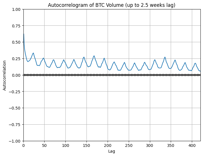
Generate an autocorrelogram graph for the BTC volume data.
!pip install numpy pandas keras seaborn matplotlib temporal_linear_network scikit-learn jax
/home/remi/.pyenv/versions/3.12.3/lib/python3.12/pty.py:95: RuntimeWarning: os.fork() was called. os.fork() is incompatible with multithreaded code, and JAX is multithreaded, so this will likely lead to a deadlock.
  pid, fd = os.forkpty()
WARNING: Ignoring invalid distribution ~umpy (/home/remi/.pyenv/versions/3.12.3/lib/python3.12/site-packages)
WARNING: Ignoring invalid distribution ~umpy (/home/remi/.pyenv/versions/3.12.3/lib/python3.12/site-packages)
Requirement already satisfied: numpy in /home/remi/.pyenv/versions/3.12.3/lib/python3.12/site-packages (2.2.0)
Requirement already satisfied: pandas in /home/remi/.pyenv/versions/3.12.3/lib/python3.12/site-packages (2.2.3)
Requirement already satisfied: keras in /home/remi/.pyenv/versions/3.12.3/lib/python3.12/site-packages (3.8.0)
Requirement already satisfied: seaborn in /home/remi/.pyenv/versions/3.12.3/lib/python3.12/site-packages (0.13.2)
Requirement already satisfied: matplotlib in /home/remi/.pyenv/versions/3.12.3/lib/python3.12/site-packages (3.10.0)
Requirement already satisfied: temporal_linear_network in /home/remi/.pyenv/versions/3.12.3/lib/python3.12/site-packages (0.1.2)
Requirement already satisfied: scikit-learn in /home/remi/.pyenv/versions/3.12.3/lib/python3.12/site-packages (1.6.1)
Requirement already satisfied: jax in /home/remi/.pyenv/versions/3.12.3/lib/python3.12/site-packages (0.5.0)
Requirement already satisfied: python-dateutil>=2.8.2 in /home/remi/.pyenv/versions/3.12.3/lib/python3.12/site-packages (from pandas) (2.9.0.post0)
Requirement already satisfied: pytz>=2020.1 in /home/remi/.pyenv/versions/3.12.3/lib/python3.12/site-packages (from pandas) (2024.2)
Requirement already satisfied: tzdata>=2022.7 in /home/remi/.pyenv/versions/3.12.3/lib/python3.12/site-packages (from pandas) (2024.2)
Requirement already satisfied: absl-py in /home/remi/.pyenv/versions/3.12.3/lib/python3.12/site-packages (from keras) (2.1.0)
Requirement already satisfied: rich in /home/remi/.pyenv/versions/3.12.3/lib/python3.12/site-packages (from keras) (13.9.4)
Requirement already satisfied: namex in /home/remi/.pyenv/versions/3.12.3/lib/python3.12/site-packages (from keras) (0.0.8)
Requirement already satisfied: h5py in /home/remi/.pyenv/versions/3.12.3/lib/python3.12/site-packages (from keras) (3.12.1)
Requirement already satisfied: optree in /home/remi/.pyenv/versions/3.12.3/lib/python3.12/site-packages (from keras) (0.14.0)
Requirement already satisfied: ml-dtypes in /home/remi/.pyenv/versions/3.12.3/lib/python3.12/site-packages (from keras) (0.4.1)
Requirement already satisfied: packaging in /home/remi/.local/lib/python3.12/site-packages (from keras) (23.2)
Requirement already satisfied: contourpy>=1.0.1 in /home/remi/.pyenv/versions/3.12.3/lib/python3.12/site-packages (from matplotlib) (1.3.1)
Requirement already satisfied: cycler>=0.10 in /home/remi/.pyenv/versions/3.12.3/lib/python3.12/site-packages (from matplotlib) (0.12.1)
Requirement already satisfied: fonttools>=4.22.0 in /home/remi/.pyenv/versions/3.12.3/lib/python3.12/site-packages (from matplotlib) (4.55.8)
Requirement already satisfied: kiwisolver>=1.3.1 in /home/remi/.pyenv/versions/3.12.3/lib/python3.12/site-packages (from matplotlib) (1.4.8)
Requirement already satisfied: pillow>=8 in /home/remi/.pyenv/versions/3.12.3/lib/python3.12/site-packages (from matplotlib) (11.1.0)
Requirement already satisfied: pyparsing>=2.3.1 in /home/remi/.pyenv/versions/3.12.3/lib/python3.12/site-packages (from matplotlib) (3.2.1)
Requirement already satisfied: scipy>=1.6.0 in /home/remi/.pyenv/versions/3.12.3/lib/python3.12/site-packages (from scikit-learn) (1.15.1)
Requirement already satisfied: joblib>=1.2.0 in /home/remi/.local/lib/python3.12/site-packages (from scikit-learn) (1.3.2)
Requirement already satisfied: threadpoolctl>=3.1.0 in /home/remi/.local/lib/python3.12/site-packages (from scikit-learn) (3.2.0)
Requirement already satisfied: jaxlib<=0.5.0,>=0.5.0 in /home/remi/.pyenv/versions/3.12.3/lib/python3.12/site-packages (from jax) (0.5.0)
Requirement already satisfied: opt_einsum in /home/remi/.local/lib/python3.12/site-packages (from jax) (3.3.0)
Requirement already satisfied: six>=1.5 in /home/remi/.pyenv/versions/3.12.3/lib/python3.12/site-packages (from python-dateutil>=2.8.2->pandas) (1.16.0)
Requirement already satisfied: typing-extensions>=4.5.0 in /home/remi/.pyenv/versions/3.12.3/lib/python3.12/site-packages (from optree->keras) (4.12.2)
Requirement already satisfied: markdown-it-py>=2.2.0 in /home/remi/.pyenv/versions/3.12.3/lib/python3.12/site-packages (from rich->keras) (3.0.0)
Requirement already satisfied: pygments<3.0.0,>=2.13.0 in /home/remi/.pyenv/versions/3.12.3/lib/python3.12/site-packages (from rich->keras) (2.18.0)
Requirement already satisfied: mdurl~=0.1 in /home/remi/.pyenv/versions/3.12.3/lib/python3.12/site-packages (from markdown-it-py>=2.2.0->rich->keras) (0.1.2)
WARNING: Ignoring invalid distribution ~umpy (/home/remi/.pyenv/versions/3.12.3/lib/python3.12/site-packages)
WARNING: Ignoring invalid distribution ~umpy (/home/remi/.pyenv/versions/3.12.3/lib/python3.12/site-packages)

[notice] A new release of pip is available: 24.3.1 -> 25.0.1
[notice] To update, run: pip install --upgrade pip
import osBACKEND ='jax'# You can use any backend hereos.environ['KERAS_BACKEND'] = BACKENDimport timeimport numpy as npimport pandas as pdfrom keras import Modelfrom keras.layers import Denseimport kerasimport pandas as pdfrom pandas.plotting import autocorrelation_plotimport seaborn as snsimport matplotlib.pyplot as pltfrom tln import TLNfrom sklearn.metrics import r2_scorefrom sklearn.linear_model import LinearRegressionkeras.utils.set_random_seed(1) N_MAX_EPOCHS =1000BATCH_SIZE =128early_stopping_callback =lambda : keras.callbacks.EarlyStopping( monitor="val_loss", min_delta=0.00001, patience=10, mode="min", restore_best_weights=True, start_from_epoch=6,)lr_callback =lambda : keras.callbacks.ReduceLROnPlateau( monitor="val_loss", factor=0.25, patience=5, mode="min", min_delta=0.00001, min_lr=0.000025, verbose=0,)callbacks =lambda : [early_stopping_callback(), lr_callback(), keras.callbacks.TerminateOnNaN()]NOTIONAL_PARQUET_PATH ="hourly_notionals.parquet"VOLUME_PARQUET_PATH ="hourly_volumes.parquet"
# 1. Load the data using pd.read_parquetdf_notional = pd.read_parquet(NOTIONAL_PARQUET_PATH)df_volume = pd.read_parquet(VOLUME_PARQUET_PATH)# Filter data for BTC only (assuming the BTC column exists)btc_notional = df_notional['BTC']btc_volume = df_volume['BTC']# 2. Compute the VWAP for each time point (VWAP = notional / volume)# Use forward fill to handle any NaN values.vwap = btc_notional / btc_volumevwap = vwap.fillna(method='ffill')# 3. Compute returns over time using VWAP as the pricereturns = vwap.pct_change()# 4. Create a scatter plot of volume vs. absolute returns (both axes in log scale)plt.figure(figsize=(8,6))plt.scatter(btc_volume, returns.abs(), alpha=0.5)plt.xscale('log')plt.yscale('log')plt.xlabel("Volume (log scale)")plt.ylabel("Absolute Return (log scale)")plt.title("Scatter Plot: Volume vs. Absolute Return")plt.show()# 5. Compute the average volume for each hour of the day and plot it# Hint: Create a column 'Hour' from the datetime index and group by this column.btc_volume_df = btc_volume.to_frame(name='Volume')btc_volume_df['Hour'] = btc_volume_df.index.houravg_volume_by_hour = btc_volume_df.groupby('Hour')['Volume'].mean()plt.figure(figsize=(8,6))avg_volume_by_hour.plot(kind='bar', color='skyblue')plt.xlabel("Hour of the Day")plt.ylabel("Average Volume")plt.title("Average Volume by Hour of the Day")plt.show()# 6. Create an autocorrelogram of the BTC volume limited to 2.5 weeks (420 hours)plt.figure(figsize=(8,6))autocorrelation_plot(btc_volume)plt.xlim(0, 420) # Limit lags to 420 hoursplt.title("Autocorrelogram of BTC Volume (up to 2.5 weeks lag)")plt.show()
/tmp/ipykernel_2719374/3340261912.py:12: FutureWarning: Series.fillna with 'method' is deprecated and will raise in a future version. Use obj.ffill() or obj.bfill() instead.
  vwap = vwap.fillna(method='ffill')
TP Part 2: Setting the Problem and Creating Our Naive Benchmark
Problem Statement
Our goal is to execute a 12-hour VWAP (Volume-Weighted Average Price) order. To do so, we need to determine how to allocate our trading volume over a 12-hour period.
A common benchmark for order execution is the TWAP (Time-Weighted Average Price). TWAP is defined as the simple (arithmetic) average price over a given period. For a 12-hour TWAP, the naive approach is to allocate the order equally over each hour; that is, you assign an equal weight of 1/12 to each of the 12 bins.
Our objective is to quantify the deviation between this naive TWAP benchmark and the real VWAP (which takes volume into account). To achieve this, we will perform the following steps for each 12-hour window in our dataset:
Compute the VWAP over 12 hours:
For each 12-hour window, compute the VWAP as:
This corresponds to allocating 1/12 of the order to each hour.
Quantify the Deviation:
Compare the TWAP and VWAP for each window by computing a deviation (for example, the absolute difference). This will help us assess how much the naive equal allocation (TWAP) deviates from the more realistic VWAP, which accounts for volume differences.
Building the Matrices
To perform the above calculations for each 12-hour window, we need to reshape our data into matrices of shape (num_elements - 12, 12), where each row represents a 12-hour window: - One matrix will hold the VWAP values for each window. - Another matrix will hold the corresponding volume values.
With these matrices, we can compute: - VWAP for each window:
Multiply the VWAP values by the corresponding volume values, sum them along each row, and divide by the sum of volumes in that row. - TWAP for each window:
Compute the arithmetic mean of the VWAP values in each row (since each hour receives an equal weight of 1/12).
# Define data pathsNOTIONAL_PARQUET_PATH ="hourly_notionals.parquet"VOLUME_PARQUET_PATH ="hourly_volumes.parquet"# 1. Load the datadf_notional = pd.read_parquet(NOTIONAL_PARQUET_PATH)df_volume = pd.read_parquet(VOLUME_PARQUET_PATH)# Filter for BTC data (assume the BTC column exists)btc_notional = df_notional['BTC']btc_volume = df_volume['BTC']# Compute per-hour VWAP (notional divided by volume) and handle missing values by forward fillingvwap = (btc_notional / btc_volume).fillna(method='ffill')# Set window parameters for a 12-hour periodwindow_size =12N =len(vwap)num_windows = N - window_size +1# 2. Create matrices for each 12-hour windowvwap_matrix = np.array([vwap.iloc[i:i+window_size].values for i inrange(num_windows)])volume_matrix = np.array([btc_volume.iloc[i:i+window_size].values for i inrange(num_windows)])# 3. Compute the VWAP for each windowVWAP_window = (vwap_matrix * volume_matrix).sum(axis=1) / volume_matrix.sum(axis=1)# 4. Compute the TWAP for each window (equal weighting: 1/12 per bin)TWAP_window = vwap_matrix.mean(axis=1)# 5. Compute the absolute deviation between TWAP and VWAP in proportion deviation = np.abs(VWAP_window / TWAP_window -1)# 6. Output the mean deviation as a naive benchmark metricprint("Mean Absolute Deviation between TWAP and VWAP:", deviation.mean())
/tmp/ipykernel_2719374/2533258188.py:14: FutureWarning: Series.fillna with 'method' is deprecated and will raise in a future version. Use obj.ffill() or obj.bfill() instead.
  vwap = (btc_notional / btc_volume).fillna(method='ffill')
Mean Absolute Deviation between TWAP and VWAP: 0.0018336970878729138
Using Historical Data for Volume Allocation
In order to optimally allocate our trading volume over time (in our case, over a 12-hour VWAP window), we typically want to build a model that learns from historical market data. The idea is to use past observations to predict future behavior, allowing our model to decide how much volume to allocate in each future time step. The overall process includes:
Creating the Input (X) Matrix:
We extract features from historical data (such as past volumes, VWAP values, time-of-day, day-of-week, and returns). These features are collected over a defined “lookback” window (for example, the previous 120 hours). This matrix represents the state of the market in the past.
Creating the Target (y) Matrix:
We then create targets that represent the future we want to predict—in this case, the future VWAP and volume over the next few hours (for example, the next 12 hours). Often, we also apply scaling to these targets so that the model learns relative changes rather than absolute values.
Splitting the Data:
To evaluate the performance of our model, we split the dataset into training and test sets. The training set is used to build the model, while the test set is reserved for evaluating its performance on unseen data.
This process ensures that our model is provided with a clear, historical context (via the X matrix) and is trained to predict the outcomes it needs to manage the order execution effectively (via the y matrix).
Explanation of the Given Functions
We now present two functions that implement the above steps:
prepare_data Function
This function creates the input (X) and target (y) matrices from the raw VWAP and volume data along with additional features. Its key steps are:
Sliding Window Extraction:
It moves through the dataset with a sliding window approach. For each position, the past lookback hours of features are collected into a row of the X matrix.
Target Construction:
For the corresponding target, it collects the next n_ahead hours of VWAP and volume data. If autoscale_target is set to True, the function scales the target values based on the historical data (e.g., dividing future prices by the last price in the lookback period and normalizing volumes by the sum over the lookback window).
Concatenation and Output:
The function finally concatenates the target values for prices and volumes along the last axis and returns the X and y matrices.
full_generate Function
This function reads the raw data from our parquet files and prepares everything for modeling:
Data Loading:
It loads the volume and notional data, filters for the target asset (e.g., BTC), and computes the VWAP as the ratio of notional to volume (with forward fill applied to handle missing values).
Feature Engineering:
It creates additional features such as:
A relative volume indicator (volume divided by a rolling average).
Temporal features like the hour of the day and the day of the week.
Returns computed from the VWAP.
Data Alignment:
The function ensures that all the series are aligned and that any NaN values are handled appropriately.
Preparing Input and Targets:
It calls the prepare_data function with the processed VWAP, volume, and feature arrays, along with the specified lookback and forecast horizons.
Train-Test Split:
Finally, it splits the resulting dataset into training and testing sets based on a given test split proportion.
Understanding the Target Format and Loss Functions
Our target data, y, is a NumPy array with shape (n_samples, n_ahead, 2). For each sample (i.e., each sliding window), we have a forecast horizon of n_ahead time steps and two channels:
Channel 0: The volume for each future time step.
Channel 1: The market VWAP (price) for each future time step.
Our model predicts an allocation of volume over the forecast horizon, and we use these predictions (from y_pred[..., 0]) together with the market data (from y_true) to compute our losses.
We define three loss functions:
Quadratic VWAP Loss:
This loss calculates the squared relative deviation between the achieved VWAP and the market VWAP. The achieved VWAP is computed as a weighted average of the market VWAP using the predicted volume weights:
where \[\hat{v}_i\] is the predicted volume (from y_pred[..., 0]) and \[p_i\] is the market VWAP (from y_true[..., 1]).
The market VWAP is computed using the actual volume:
and the quadratic loss is the mean of the squared differences.
Absolute VWAP Loss:
This is similar to the quadratic loss but uses the absolute value of the relative deviation rather than its square.
Volume Curve Loss:
This loss compares the normalized (or relative) volume curves. The achieved volume curve is obtained by normalizing the predicted volumes so that they sum to one:
The loss is then the mean of the squared differences between these curves.
def quadratic_vwap_loss(y_true, y_pred):""" Computes the mean squared relative deviation between the achieved VWAP and the market VWAP. y_true: numpy array of shape (n_samples, n_ahead, 2) Channel 0 is volume, channel 1 is market VWAP. y_pred: numpy array of shape (n_samples, n_ahead, 2) We only use channel 0 (predicted volume allocation); the price is taken from y_true. """# Compute achieved VWAP as weighted average of market VWAP using predicted volumes. vwap_achieved = np.sum(y_pred[..., 0] * y_true[..., 1], axis=1) / np.sum(y_pred[..., 0], axis=1)# Compute market VWAP using actual volumes. vwap_mkt = np.sum(y_true[..., 0] * y_true[..., 1], axis=1) / np.sum(y_true[..., 0], axis=1)# Compute relative deviation. vwap_diff = vwap_achieved / vwap_mkt -1.0# Compute quadratic loss (mean squared error). loss = np.mean(np.square(vwap_diff))return lossdef absolute_vwap_loss(y_true, y_pred):""" Computes the mean absolute relative deviation between the achieved VWAP and the market VWAP. y_true: numpy array of shape (n_samples, n_ahead, 2) y_pred: numpy array of shape (n_samples, n_ahead, 2) """ vwap_achieved = np.sum(y_pred[..., 0] * y_true[..., 1], axis=1) / np.sum(y_pred[..., 0], axis=1) vwap_mkt = np.sum(y_true[..., 0] * y_true[..., 1], axis=1) / np.sum(y_true[..., 0], axis=1) vwap_diff = vwap_achieved / vwap_mkt -1.0 loss = np.mean(np.abs(vwap_diff))return lossdef volume_curve_loss(y_true, y_pred):""" Computes the mean squared error between the normalized volume curves of the prediction and the market. y_true: numpy array of shape (n_samples, n_ahead, 2) Channel 0 is volume. y_pred: numpy array of shape (n_samples, n_ahead, 2) Channel 0 is the predicted volume allocation. """# Normalize predicted volumes (achieved volume curve). volume_curve_achieved = y_pred[..., 0] / np.sum(y_pred[..., 0], axis=1, keepdims=True)# Normalize market volumes (market volume curve). volume_curve_mkt = y_true[..., 0] / np.sum(y_true[..., 0], axis=1, keepdims=True)# Compute the difference between the two curves. volume_curve_diff = volume_curve_achieved - volume_curve_mkt# Compute the loss as the mean squared error. loss = np.mean(np.square(volume_curve_diff))return loss
Recap
y_true is a NumPy array with shape (n_samples, n_ahead, 2):
Channel 0: Actual volume.
Channel 1: Market VWAP.
y_pred is expected to have the same shape, but for our purposes, we only use the predicted volumes in channel 0. The price (VWAP) comes from y_true.
These functions compute: - The quadratic VWAP loss (mean squared relative error), - The absolute VWAP loss (mean absolute relative error), and - The volume curve loss (mean squared error between normalized volume distributions).
Exercise: Evaluating Loss Functions
Now that we’ve defined our loss functions (quadratic VWAP loss, absolute VWAP loss, and volume curve loss), it’s time to test them.
Recall that our target variable y_true has shape (n_samples, n_ahead, 2), where: - Channel 0 contains the actual volumes. - Channel 1 contains the market VWAP (prices).
We want to compare two simple scenarios: 1. Naive Prediction (TWAP-like):
Here, we assume a constant predicted volume allocation over the forecast horizon. This is implemented by setting y_pred = np.ones_like(y_true)
which, when normalized, assigns an equal fraction (1/n_ahead) to each time step.
Perfect Prediction:
In this case, we simply set y_pred = y_true
so that our predictions exactly match the true values. This should result in zero loss for all our metrics.
Use the following code in a new cell to compute and print the loss values:
With y_pred = ones, you are simulating a naive constant allocation strategy (similar to TWAP). The losses computed here will quantify the deviation between this naive strategy and the actual market VWAP and volume curve.
With y_pred = y_true, the prediction is perfect, so the losses should be near zero. This serves as a sanity check for your loss functions.
Run this cell to see how the loss functions respond under both scenarios.
Exercise: Fitting a Linear Regression Model for Volume Allocation
In this exercise, you’ll fit a linear regression model from scikit-learn to predict the future volume allocation. Remember that:
Input Dimensions:
Your training input X_train has shape (n_samples, lookback, n_features), but scikit-learn models require a 2D array. Therefore, you’ll need to flatten the last two dimensions (i.e., reshape X_train to (n_samples, lookback * n_features)).
Target Dimensions:
Your target variable y_train has shape (n_samples, n_ahead, 2). Here, the first channel (i.e., y_train[..., 0]) contains the actual volumes. We will only predict this volume channel.
Post-Processing Predictions:
After prediction, you must clip the predictions to ensure they are non-negative (since negative volume allocations don’t make sense). Then, you should normalize each prediction vector so that the sum is 1 (i.e., forming a valid allocation probability distribution). In the event that the sum is 0, you should assign a uniform distribution (1/n for each of the n_ahead time steps).
Your task is to fit a linear regression model on the training data and then use it to predict y_test. Finally, add a dummy price channel (all zeros) to your predictions so that they match the target format (which has two channels: volume and price) and compute the losses as before.
# --- Step 1: Flatten the Input ---# Linear Regression requires a 2D input, so flatten the lookback and feature dimensions.X_train_flat = X_train.reshape(X_train.shape[0], -1)X_test_flat = X_test.reshape(X_test.shape[0], -1)# --- Step 2: Prepare the Target ---# Use only the first channel of y_train (the volume) as the target.y_train_volume = y_train[..., 0] # Shape: (n_samples, n_ahead)# --- Step 3: Fit the Linear Regression Model ---model = LinearRegression()model.fit(X_train_flat, y_train_volume)# --- Step 4: Predict on the Test Set ---y_pred = model.predict(X_test_flat) # Shape: (n_samples, n_ahead)# --- Step 5: Post-Process the Predictions ---# Clip negative predictions to 0 (negative volume doesn't make sense).y_pred = np.clip(y_pred, 0, None)# Normalize each prediction row so that the sum equals 1.# If the sum of a row is 0, assign a uniform distribution (1/n_ahead per step).n_ahead = y_pred.shape[1]y_pred_norm = np.zeros_like(y_pred)for i inrange(y_pred.shape[0]): row_sum = y_pred[i].sum()if row_sum >0: y_pred_norm[i] = y_pred[i] / row_sumelse: y_pred_norm[i] = np.ones(n_ahead) / n_ahead# --- Step 6: Expand the Prediction to Match Target Format ---# The target y has shape (n_samples, n_ahead, 2) where:# - Channel 0 is volume.# - Channel 1 is market VWAP (price).# Since our model predicts only volumes, add a dummy price channel (filled with zeros).y_pred_expanded = np.expand_dims(y_pred_norm, axis=-1) # Now shape becomes (n_samples, n_ahead, 1)dummy_price_channel = np.zeros_like(y_pred_expanded)y_pred_expanded = np.concatenate([y_pred_expanded, dummy_price_channel], axis=-1) # Final shape: (n_samples, n_ahead, 2)# --- Step 7: Compute Losses ---quad_loss = quadratic_vwap_loss(y_test, y_pred_expanded)abs_loss = absolute_vwap_loss(y_test, y_pred_expanded)vol_loss = volume_curve_loss(y_test, y_pred_expanded)print("Losses for the Linear Regression model:")print("Quadratic VWAP Loss:", quad_loss)print("Absolute VWAP Loss:", abs_loss)print("Volume Curve Loss:", vol_loss)
Losses for the Linear Regression model:
Quadratic VWAP Loss: 8.131472516180487e-06
Absolute VWAP Loss: 0.0014428517510359324
Volume Curve Loss: 0.002661528628047214
Deep Learning Approach for VWAP Allocation
Now that we have our baseline with linear regression, we move on to a deep learning approach. Deep learning is very attractive for this problem because it acts as a general function calibrator: it can approximate any differentiable function when optimized end‐to‐end. Our loss functions (quadratic VWAP loss, absolute VWAP loss, and volume curve loss) are all differentiable. By replacing NumPy operations with Keras3 operations—and with our backend set to JAX—we enable automatic differentiation (AD). This means that every tensor operation (sums, means, softmax, etc.) is tracked for gradient computation, allowing us to update our model parameters via gradient descent.
Keras3 with JAX and the TLN Package
We use Keras3 for its backend agnosticism and set the backend to JAX for fast, compiled, and automatically differentiable operations. In our model, we import the Temporal Linear Network (TLN) as a package. TLN is a fully linear model designed for deep learning on time series data. In simple terms, TLN is a fully linear network that processes sequential inputs; it is very efficient and interpretable, and you can find more details in the paper https://arxiv.org/abs/2410.21448.
How a Model is Created in Keras
When building a model in Keras, you typically define: - The __init__ method: Initialize parameters and sub-layers. - The build method: Create weights based on the input shape. - The call method: Define the forward pass of the model.
Our StaticVWAP Model
Our goal is to learn an allocation for future volume over n_ahead time steps from past data. The model should output a vector of length n_ahead that sums to 1 (a valid order allocation). We enforce this using a softmax operation. Since our target format is (batch_size, n_ahead, 2)—with the first channel for volume and the second for price—we add a dummy price channel (all zeros) to the model’s output.
class StaticVWAP(keras.Model):def__init__(self, lookback, n_ahead, internal_model=None):super(StaticVWAP, self).__init__()self.lookback = lookbackself.n_ahead = n_ahead# Use TLN as our internal model. TLN is a fully linear time series model.# For more details, see: https://arxiv.org/abs/2410.21448self.internal_model = internal_model if internal_model isnotNoneelse TLN( output_len=n_ahead, output_features=1, flatten_output=False, hidden_layers=2, use_convolution=True, name='TLN' )def build(self, input_shape):# input_shape is (batch_size, lookback, n_features) internal_model_input_shape = (input_shape[0], self.lookback, input_shape[2])self.internal_model.build(internal_model_input_shape)super(StaticVWAP, self).build(input_shape)def call(self, inputs):# Process inputs through the internal model to obtain raw outputs. preds =self.internal_model(inputs) # Expected shape: (batch_size, n_ahead, 1)# Apply softmax along the time axis (n_ahead) to ensure the allocations are non-negative and sum to 1. volume_curve = keras.ops.softmax(preds, axis=1)# Create a dummy price channel (all zeros) so the output shape matches our target: (batch_size, n_ahead, 2) dummy_price_channel = keras.ops.zeros_like(preds) results = keras.ops.concatenate([volume_curve, dummy_price_channel], axis=-1)return resultsdef keras_absolute_vwap_loss(y_true, y_pred):""" Computes the mean absolute relative deviation between the achieved VWAP and the market VWAP. y_true: numpy array of shape (n_samples, n_ahead, 2) y_pred: numpy array of shape (n_samples, n_ahead, 2) """ vwap_achieved = keras.ops.sum(y_pred[..., 0] * y_true[..., 1], axis=1) / keras.ops.sum(y_pred[..., 0], axis=1) vwap_mkt = keras.ops.sum(y_true[..., 0] * y_true[..., 1], axis=1) / keras.ops.sum(y_true[..., 0], axis=1) vwap_diff = vwap_achieved / vwap_mkt -1.0 loss = keras.ops.mean(keras.ops.abs(vwap_diff))return lossdef keras_volume_curve_loss(y_true, y_pred):""" Computes the mean squared error between the normalized volume curves of the prediction and the market. y_true: numpy array of shape (n_samples, n_ahead, 2) Channel 0 is volume. y_pred: numpy array of shape (n_samples, n_ahead, 2) Channel 0 is the predicted volume allocation. """# Normalize predicted volumes (achieved volume curve). volume_curve_achieved = y_pred[..., 0] / keras.ops.sum(y_pred[..., 0], axis=1, keepdims=True)# Normalize market volumes (market volume curve). volume_curve_mkt = y_true[..., 0] / keras.ops.sum(y_true[..., 0], axis=1, keepdims=True)# Compute the difference between the two curves. volume_curve_diff = volume_curve_achieved - volume_curve_mkt# Compute the loss as the mean squared error. loss = keras.ops.mean(keras.ops.square(volume_curve_diff))return loss
Training and Evaluating the StaticVWAP Model
In this section, we will train our deep learning model (StaticVWAP) to learn the optimal volume allocation for VWAP execution. Our approach is to directly minimize differentiable loss functions that capture the quality of the execution, such as:
Absolute VWAP Loss: Measures the mean absolute relative deviation between the achieved VWAP (using the predicted volume allocation) and the market VWAP.
Volume Curve Loss: Measures the mean squared error between the normalized predicted volume curve and the actual market volume distribution.
For both trainings, we use the following hyperparameters and callbacks: - Maximum Epochs:N_MAX_EPOCHS = 1000 - Batch Size:BATCH_SIZE = 128 - Early Stopping Callback: Monitors val_loss with a minimum change of 0.00001 and stops if no improvement is observed for 10 epochs (starting from epoch 6). It also restores the best weights. - Learning Rate Callback: Reduces the learning rate by a factor of 0.25 if the validation loss does not improve for 5 epochs, with a minimum learning rate of 0.000025. - Terminate on NaN: Stops training if any NaN values occur during training.
After training, we evaluate our model on the test set by computing: - Absolute VWAP Loss - Quadratic VWAP Loss (a related metric) - R2 Volume Curve Score: Calculated on the normalized volume curves.
For comparison, we also define a naive prediction that assigns a uniform allocation (i.e., 1/n_ahead for each of the n_ahead time steps).
Below is the code that trains the model with each loss function and evaluates its performance:
Callbacks & Hyperparameters:
We set up early stopping, learning rate reduction, and a termination callback to ensure efficient and stable training.
Model Compilation:
The StaticVWAP model is compiled with the Adam optimizer. In the first training run, we use the absolute VWAP loss as our primary loss function and volume curve loss as a metric. In the second training run, we swap these roles by using the volume curve loss as the primary loss.
Training:
The model is trained on X_train and y_train with a validation split. The training history and total training time are recorded.
Evaluation:
After training, we predict on X_test and evaluate the predictions using our custom loss functions and an R2 score computed on the normalized volume curves.
This approach demonstrates how deep learning can be applied to directly optimize the execution objective by leveraging differentiable loss functions, backend-agnostic operations (with Keras3 and JAX), and a model architecture (StaticVWAP) that outputs a valid volume allocation distribution.