import pandas as pd
import numpy as np
import matplotlib.pyplot as plt
import yfinance as yf
from scipy.optimize import minimize
import seaborn as snsModern Portfolio Theory - Practical Work - Corrected version
L3 Finance
Part 1: Data Retrieval and Initial Processing
Question 1.1
We will work with a diversified portfolio of major stocks covering different sectors of the economy. Using the yfinance library, retrieve daily closing prices for the following stocks from January 1st, 2015 to January 1st, 2025:
Hint: Use yf.download() function with parameters: - tickers: list or string of tickers - start: start date - end: end date - interval: ‘d’ for daily data - Use the ‘Close’ column
# Define the tickers
tickers = [
    # Technology
    'AAPL', 'MSFT', 'INTC', 'CSCO', 'ORCL',
    # Financial Services
    'JPM', 'BAC', 'GS', 'MS', 'C', 'AXP', 'WFC',
    # Healthcare
    'JNJ', 'PFE', 'MRK', 'ABT', 'BMY',
    # Energy
    'XOM', 'CVX', 'COP', 'SLB', 'OXY',
    # Consumer Staples
    'WMT', 'PG', 'KO', 'PEP', 'CL', 'KMB', 'GIS',
    # Consumer Discretionary
    'HD', 'MCD', 'NKE', 'SBUX', 'TJX', 'LOW', 'YUM',
    # Industrial
    'CAT', 'BA', 'MMM', 'HON', 'GE', 'DE', 'FDX',
    # Materials
    'APD', 'ECL', 'NEM', 'FCX', 'PPG', 'NUE',
    # Telecommunications
    'VZ', 'T', 'CMCSA',
    # Real Estate
    'SPG', 'PSA'
]


# Download the data
start_date = '2010-01-01'
end_date = '2025-01-01'

prices = yf.download(tickers,
                    start=start_date,
                    end=end_date,
                    interval='1d')['Close']

# Check the first few rows of the data
print("First few rows of the price data:")
print(prices.head())
[*********************100%***********************] 54 of 54 completedFirst few rows of the price data:
Ticker AAPL ABT APD AXP BA BAC \
Date
2010-01-04 6.447412 18.665758 52.804508 32.828983 43.777561 12.451034
2010-01-05 6.458560 18.514959 52.366360 32.756783 45.211349 12.855753
2010-01-06 6.355827 18.617779 51.934586 33.286285 46.582794 13.006530
2010-01-07 6.344077 18.772020 51.636158 33.826145 48.468563 13.435059
2010-01-08 6.386254 18.867979 51.966351 33.801979 48.001026 13.316021
Ticker BMY C CAT CL ... SBUX \
Date ...
2010-01-04 15.436789 25.928009 39.738235 28.930437 ... 8.835545
2010-01-05 15.195873 26.919380 40.213326 29.164408 ... 9.042539
2010-01-06 15.189850 27.758226 40.335484 29.098055 ... 8.977375
2010-01-07 15.201899 27.834469 40.498383 28.982828 ... 8.954374
2010-01-08 14.948930 27.376934 40.953117 28.462532 ... 8.923708
Ticker SLB SPG T TJX VZ WFC \
Date
2010-01-04 47.246723 39.174126 7.038978 7.384900 14.442019 18.417709
2010-01-05 47.380508 38.906082 7.004502 7.583662 14.468057 18.923317
2010-01-06 48.436508 38.469257 6.935692 7.614400 14.052043 18.950285
2010-01-07 48.936378 38.970608 6.857815 8.003725 13.968397 19.637922
2010-01-08 49.738956 38.037426 6.807579 7.899220 13.977206 19.455894
Ticker WMT XOM YUM
Date
2010-01-04 13.084426 39.272114 18.878279
2010-01-05 12.954136 39.425453 18.813725
2010-01-06 12.925184 39.766212 18.679226
2010-01-07 12.932426 39.641270 18.673841
2010-01-08 12.867274 39.482235 18.679226
[5 rows x 54 columns]Question 1.2
Calculate the daily returns for each asset. The daily return is defined as the percentage change in price from one day to the next.
Hint: - Use the pct_change() method from pandas - Be sure to handle any missing values that might appear
# Calculate daily returns
returns = prices.pct_change()

# Drop any missing values
returns = returns.dropna()

# Display summary statistics of the returns
print("\nSummary statistics of daily returns:")
print(returns.describe())
Summary statistics of daily returns:
Ticker         AAPL          ABT          APD          AXP           BA  \
count   3773.000000  3773.000000  3773.000000  3773.000000  3773.000000
mean       0.001124     0.000568     0.000567     0.000748     0.000625
std        0.017552     0.013505     0.015242     0.018248     0.022538
min       -0.128647    -0.097857    -0.155518    -0.148187    -0.238484
25%       -0.007398    -0.006053    -0.006462    -0.007042    -0.009198
50%        0.001001     0.000596     0.000751     0.000768     0.000676
75%        0.010355     0.007639     0.008000     0.009271     0.010452
max        0.119808     0.109360     0.137233     0.218822     0.243186

Ticker          BAC          BMY            C          CAT           CL  ...  \
count   3773.000000  3773.000000  3773.000000  3773.000000  3773.000000  ...
mean       0.000559     0.000449     0.000494     0.000753     0.000365  ...
std        0.021172     0.014655     0.021367     0.018295     0.011262  ...
min       -0.203182    -0.159851    -0.192986    -0.142822    -0.097829  ...
25%       -0.009895    -0.006971    -0.009486    -0.008498    -0.005121  ...
50%        0.000349     0.000622     0.000294     0.000584     0.000369  ...
75%        0.010749     0.007588     0.010222     0.010267     0.006184  ...
max        0.177962     0.114425     0.179843     0.103321     0.126082  ...

Ticker         SBUX          SLB          SPG            T          TJX  \
count   3773.000000  3773.000000  3773.000000  3773.000000  3773.000000
mean       0.000768     0.000208     0.000605     0.000392     0.000864
std        0.017326     0.022881     0.020546     0.012944     0.015659
min       -0.162042    -0.274214    -0.267127    -0.104061    -0.203995
25%       -0.007363    -0.010883    -0.007593    -0.005913    -0.006955
50%        0.000654    -0.000108     0.000992     0.000725     0.000714
75%        0.008734     0.010998     0.009068     0.006838     0.008502
max        0.244970     0.199080     0.278694     0.100223     0.129033

Ticker           VZ          WFC          WMT          XOM          YUM
count   3773.000000  3773.000000  3773.000000  3773.000000  3773.000000
mean       0.000333     0.000532     0.000585     0.000391     0.000631
std        0.011605     0.018845     0.012085     0.015723     0.014886
min       -0.074978    -0.158676    -0.113757    -0.122248    -0.188324
25%       -0.005823    -0.008342    -0.005145    -0.007267    -0.006211
50%        0.000496     0.000341     0.000679     0.000133     0.000812
75%        0.006458     0.009181     0.006373     0.007995     0.007590
max        0.092705     0.145346     0.117085     0.126868     0.232485

[8 rows x 54 columns]
Question 1.3
Create a visualization of the correlation between the assets using a heatmap. Also, compute and display the covariance matrix.
Hint: - Use seaborn.heatmap() for visualization - Use returns.corr() for correlation matrix - Use returns.cov() for covariance matrix
# Compute correlation matrix
correlation_matrix = returns.corr()

# Create a heatmap
plt.figure(figsize=(10, 8))
sns.heatmap(correlation_matrix,
            annot=False,
            cmap='coolwarm',
            vmin=-1,
            vmax=1,
            center=0)
plt.title('Correlation Matrix of Asset Returns')
plt.show()

# Compute and display covariance matrix
covariance_matrix = returns.cov()
print("\nCovariance Matrix:")
print(covariance_matrix)
Covariance Matrix:
Ticker      AAPL       ABT       APD       AXP        BA       BAC       BMY  \
Ticker
AAPL    0.000308  0.000095  0.000105  0.000131  0.000152  0.000141  0.000065
ABT     0.000095  0.000182  0.000097  0.000101  0.000103  0.000111  0.000079
APD     0.000105  0.000097  0.000232  0.000135  0.000143  0.000158  0.000073
AXP     0.000131  0.000101  0.000135  0.000333  0.000237  0.000260  0.000081
BA      0.000152  0.000103  0.000143  0.000237  0.000508  0.000236  0.000082
BAC     0.000141  0.000111  0.000158  0.000260  0.000236  0.000448  0.000091
BMY     0.000065  0.000079  0.000073  0.000081  0.000082  0.000091  0.000215
C       0.000147  0.000114  0.000162  0.000265  0.000263  0.000383  0.000097
CAT     0.000128  0.000087  0.000147  0.000187  0.000200  0.000226  0.000074
CL      0.000059  0.000069  0.000075  0.000064  0.000070  0.000067  0.000055
CMCSA   0.000103  0.000081  0.000100  0.000136  0.000133  0.000153  0.000070
COP     0.000111  0.000078  0.000134  0.000193  0.000209  0.000226  0.000081
CSCO    0.000132  0.000096  0.000110  0.000136  0.000139  0.000163  0.000073
CVX     0.000100  0.000080  0.000121  0.000171  0.000187  0.000194  0.000077
DE      0.000120  0.000085  0.000131  0.000168  0.000198  0.000198  0.000072
ECL     0.000110  0.000097  0.000131  0.000150  0.000153  0.000159  0.000071
FCX     0.000186  0.000127  0.000210  0.000263  0.000292  0.000306  0.000103
FDX     0.000127  0.000096  0.000130  0.000163  0.000193  0.000199  0.000071
GE      0.000118  0.000087  0.000128  0.000196  0.000234  0.000221  0.000074
GIS     0.000043  0.000053  0.000058  0.000041  0.000035  0.000051  0.000046
GS      0.000131  0.000099  0.000136  0.000217  0.000207  0.000297  0.000081
HD      0.000118  0.000091  0.000107  0.000134  0.000144  0.000147  0.000070
HON     0.000116  0.000094  0.000130  0.000170  0.000195  0.000188  0.000078
INTC    0.000161  0.000108  0.000125  0.000155  0.000181  0.000171  0.000069
JNJ     0.000061  0.000078  0.000072  0.000075  0.000076  0.000084  0.000071
JPM     0.000119  0.000100  0.000139  0.000225  0.000209  0.000316  0.000083
KMB     0.000050  0.000062  0.000066  0.000056  0.000055  0.000058  0.000053
KO      0.000064  0.000065  0.000077  0.000090  0.000098  0.000088  0.000053
LOW     0.000122  0.000096  0.000113  0.000146  0.000159  0.000165  0.000072
MCD     0.000078  0.000066  0.000077  0.000098  0.000110  0.000096  0.000052
MMM     0.000099  0.000085  0.000112  0.000135  0.000138  0.000157  0.000071
MRK     0.000064  0.000084  0.000078  0.000081  0.000077  0.000096  0.000076
MS      0.000151  0.000124  0.000168  0.000256  0.000237  0.000365  0.000100
MSFT    0.000166  0.000105  0.000112  0.000136  0.000139  0.000144  0.000066
NEM     0.000056  0.000040  0.000070  0.000048  0.000056  0.000044  0.000036
NKE     0.000127  0.000093  0.000109  0.000145  0.000164  0.000148  0.000066
NUE     0.000125  0.000090  0.000155  0.000192  0.000200  0.000240  0.000079
ORCL    0.000128  0.000090  0.000115  0.000135  0.000132  0.000158  0.000066
OXY     0.000125  0.000083  0.000147  0.000224  0.000272  0.000269  0.000080
PEP     0.000071  0.000069  0.000075  0.000075  0.000079  0.000078  0.000055
PFE     0.000072  0.000084  0.000082  0.000090  0.000092  0.000106  0.000090
PG      0.000063  0.000068  0.000069  0.000066  0.000066  0.000071  0.000053
PPG     0.000113  0.000095  0.000143  0.000167  0.000177  0.000187  0.000076
PSA     0.000080  0.000070  0.000084  0.000093  0.000100  0.000104  0.000056
SBUX    0.000128  0.000091  0.000119  0.000156  0.000169  0.000161  0.000069
SLB     0.000120  0.000073  0.000145  0.000219  0.000237  0.000255  0.000077
SPG     0.000112  0.000070  0.000114  0.000218  0.000260  0.000215  0.000071
T       0.000064  0.000065  0.000076  0.000099  0.000101  0.000116  0.000055
TJX     0.000102  0.000081  0.000099  0.000147  0.000168  0.000153  0.000060
VZ      0.000049  0.000057  0.000064  0.000069  0.000066  0.000083  0.000047
WFC     0.000119  0.000097  0.000138  0.000237  0.000227  0.000315  0.000085
WMT     0.000061  0.000056  0.000058  0.000056  0.000056  0.000065  0.000043
XOM     0.000085  0.000065  0.000106  0.000149  0.000169  0.000174  0.000066
YUM     0.000098  0.000079  0.000100  0.000131  0.000144  0.000134  0.000061

Ticker         C       CAT        CL  ...      SBUX       SLB       SPG  \
Ticker                                ...
AAPL    0.000147  0.000128  0.000059  ...  0.000128  0.000120  0.000112
ABT     0.000114  0.000087  0.000069  ...  0.000091  0.000073  0.000070
APD     0.000162  0.000147  0.000075  ...  0.000119  0.000145  0.000114
AXP     0.000265  0.000187  0.000064  ...  0.000156  0.000219  0.000218
BA      0.000263  0.000200  0.000070  ...  0.000169  0.000237  0.000260
BAC     0.000383  0.000226  0.000067  ...  0.000161  0.000255  0.000215
BMY     0.000097  0.000074  0.000055  ...  0.000069  0.000077  0.000071
C       0.000457  0.000233  0.000072  ...  0.000169  0.000279  0.000238
CAT     0.000233  0.000335  0.000058  ...  0.000122  0.000248  0.000160
CL      0.000072  0.000058  0.000127  ...  0.000071  0.000055  0.000064
CMCSA   0.000160  0.000127  0.000066  ...  0.000113  0.000131  0.000129
COP     0.000243  0.000216  0.000055  ...  0.000123  0.000366  0.000190
CSCO    0.000166  0.000139  0.000068  ...  0.000120  0.000141  0.000115
CVX     0.000210  0.000181  0.000058  ...  0.000111  0.000286  0.000170
DE      0.000204  0.000229  0.000061  ...  0.000119  0.000205  0.000155
ECL     0.000164  0.000131  0.000072  ...  0.000127  0.000139  0.000141
FCX     0.000327  0.000345  0.000069  ...  0.000171  0.000379  0.000240
FDX     0.000213  0.000179  0.000065  ...  0.000134  0.000177  0.000157
GE      0.000237  0.000190  0.000061  ...  0.000131  0.000222  0.000192
GIS     0.000048  0.000038  0.000068  ...  0.000045  0.000036  0.000032
GS      0.000303  0.000194  0.000061  ...  0.000139  0.000217  0.000186
HD      0.000153  0.000120  0.000070  ...  0.000127  0.000111  0.000139
HON     0.000197  0.000172  0.000066  ...  0.000127  0.000175  0.000161
INTC    0.000185  0.000155  0.000062  ...  0.000123  0.000153  0.000134
JNJ     0.000086  0.000070  0.000060  ...  0.000063  0.000068  0.000060
JPM     0.000315  0.000192  0.000065  ...  0.000139  0.000221  0.000188
KMB     0.000059  0.000049  0.000086  ...  0.000057  0.000039  0.000054
KO      0.000094  0.000074  0.000071  ...  0.000075  0.000082  0.000095
LOW     0.000173  0.000135  0.000071  ...  0.000137  0.000133  0.000157
MCD     0.000107  0.000077  0.000059  ...  0.000106  0.000088  0.000104
MMM     0.000162  0.000154  0.000065  ...  0.000101  0.000142  0.000125
MRK     0.000098  0.000078  0.000059  ...  0.000068  0.000083  0.000068
MS      0.000367  0.000232  0.000074  ...  0.000167  0.000260  0.000204
MSFT    0.000152  0.000123  0.000067  ...  0.000129  0.000107  0.000105
NEM     0.000050  0.000078  0.000038  ...  0.000045  0.000099  0.000056
NKE     0.000160  0.000129  0.000065  ...  0.000153  0.000125  0.000138
NUE     0.000252  0.000230  0.000061  ...  0.000131  0.000243  0.000180
ORCL    0.000163  0.000136  0.000068  ...  0.000117  0.000129  0.000104
OXY     0.000293  0.000244  0.000058  ...  0.000142  0.000429  0.000262
PEP     0.000081  0.000062  0.000079  ...  0.000077  0.000062  0.000075
PFE     0.000109  0.000086  0.000056  ...  0.000073  0.000084  0.000079
PG      0.000073  0.000056  0.000085  ...  0.000066  0.000050  0.000056
PPG     0.000199  0.000167  0.000068  ...  0.000129  0.000165  0.000160
PSA     0.000107  0.000084  0.000068  ...  0.000090  0.000076  0.000139
SBUX    0.000169  0.000122  0.000071  ...  0.000300  0.000134  0.000157
SLB     0.000279  0.000248  0.000055  ...  0.000134  0.000524  0.000229
SPG     0.000238  0.000160  0.000064  ...  0.000157  0.000229  0.000422
T       0.000122  0.000090  0.000059  ...  0.000072  0.000102  0.000099
TJX     0.000158  0.000120  0.000062  ...  0.000125  0.000128  0.000165
VZ      0.000083  0.000067  0.000056  ...  0.000059  0.000066  0.000071
WFC     0.000311  0.000191  0.000067  ...  0.000144  0.000229  0.000205
WMT     0.000063  0.000054  0.000057  ...  0.000060  0.000044  0.000051
XOM     0.000188  0.000166  0.000052  ...  0.000093  0.000268  0.000155
YUM     0.000144  0.000114  0.000058  ...  0.000141  0.000113  0.000129

Ticker         T       TJX        VZ       WFC       WMT       XOM       YUM
Ticker
AAPL    0.000064  0.000102  0.000049  0.000119  0.000061  0.000085  0.000098
ABT     0.000065  0.000081  0.000057  0.000097  0.000056  0.000065  0.000079
APD     0.000076  0.000099  0.000064  0.000138  0.000058  0.000106  0.000100
AXP     0.000099  0.000147  0.000069  0.000237  0.000056  0.000149  0.000131
BA      0.000101  0.000168  0.000066  0.000227  0.000056  0.000169  0.000144
BAC     0.000116  0.000153  0.000083  0.000315  0.000065  0.000174  0.000134
BMY     0.000055  0.000060  0.000047  0.000085  0.000043  0.000066  0.000061
C       0.000122  0.000158  0.000083  0.000311  0.000063  0.000188  0.000144
CAT     0.000090  0.000120  0.000067  0.000191  0.000054  0.000166  0.000114
CL      0.000059  0.000062  0.000056  0.000067  0.000057  0.000052  0.000058
CMCSA   0.000093  0.000100  0.000073  0.000139  0.000057  0.000098  0.000087
COP     0.000092  0.000115  0.000065  0.000201  0.000046  0.000263  0.000111
CSCO    0.000079  0.000102  0.000061  0.000140  0.000067  0.000103  0.000095
CVX     0.000089  0.000108  0.000067  0.000174  0.000047  0.000221  0.000102
DE      0.000085  0.000118  0.000063  0.000173  0.000055  0.000138  0.000107
ECL     0.000078  0.000115  0.000060  0.000142  0.000055  0.000102  0.000111
FCX     0.000119  0.000164  0.000083  0.000259  0.000068  0.000250  0.000165
FDX     0.000082  0.000122  0.000063  0.000173  0.000064  0.000120  0.000106
GE      0.000099  0.000133  0.000070  0.000203  0.000050  0.000153  0.000111
GIS     0.000052  0.000037  0.000050  0.000050  0.000051  0.000039  0.000040
GS      0.000097  0.000130  0.000067  0.000247  0.000056  0.000146  0.000117
HD      0.000072  0.000125  0.000060  0.000132  0.000070  0.000086  0.000104
HON     0.000085  0.000121  0.000063  0.000169  0.000055  0.000122  0.000113
INTC    0.000080  0.000112  0.000063  0.000153  0.000065  0.000111  0.000099
JNJ     0.000058  0.000058  0.000053  0.000078  0.000048  0.000062  0.000058
JPM     0.000102  0.000135  0.000074  0.000265  0.000058  0.000152  0.000119
KMB     0.000058  0.000048  0.000057  0.000055  0.000053  0.000043  0.000054
KO      0.000065  0.000070  0.000057  0.000087  0.000049  0.000071  0.000069
LOW     0.000075  0.000138  0.000060  0.000146  0.000068  0.000098  0.000112
MCD     0.000055  0.000083  0.000045  0.000092  0.000045  0.000068  0.000103
MMM     0.000076  0.000095  0.000060  0.000143  0.000052  0.000102  0.000090
MRK     0.000061  0.000062  0.000057  0.000084  0.000048  0.000070  0.000064
MS      0.000114  0.000152  0.000081  0.000293  0.000070  0.000174  0.000137
MSFT    0.000061  0.000101  0.000054  0.000124  0.000066  0.000083  0.000104
NEM     0.000047  0.000023  0.000040  0.000035  0.000029  0.000072  0.000049
NKE     0.000070  0.000130  0.000055  0.000136  0.000059  0.000094  0.000115
NUE     0.000096  0.000133  0.000077  0.000209  0.000065  0.000167  0.000115
ORCL    0.000073  0.000099  0.000057  0.000135  0.000064  0.000090  0.000089
OXY     0.000111  0.000131  0.000070  0.000243  0.000044  0.000303  0.000118
PEP     0.000061  0.000066  0.000056  0.000076  0.000060  0.000061  0.000064
PFE     0.000065  0.000065  0.000058  0.000096  0.000049  0.000072  0.000063
PG      0.000059  0.000053  0.000056  0.000068  0.000058  0.000051  0.000054
PPG     0.000078  0.000122  0.000062  0.000168  0.000049  0.000113  0.000117
PSA     0.000061  0.000080  0.000057  0.000092  0.000051  0.000064  0.000080
SBUX    0.000072  0.000125  0.000059  0.000144  0.000060  0.000093  0.000141
SLB     0.000102  0.000128  0.000066  0.000229  0.000044  0.000268  0.000113
SPG     0.000099  0.000165  0.000071  0.000205  0.000051  0.000155  0.000129
T       0.000168  0.000074  0.000101  0.000110  0.000048  0.000085  0.000063
TJX     0.000074  0.000245  0.000056  0.000143  0.000061  0.000097  0.000109
VZ      0.000101  0.000056  0.000135  0.000078  0.000046  0.000063  0.000048
WFC     0.000110  0.000143  0.000078  0.000355  0.000060  0.000162  0.000118
WMT     0.000048  0.000061  0.000046  0.000060  0.000146  0.000044  0.000045
XOM     0.000085  0.000097  0.000063  0.000162  0.000044  0.000247  0.000087
YUM     0.000063  0.000109  0.000048  0.000118  0.000045  0.000087  0.000222

[54 rows x 54 columns]
Question 1.4
Create a plot showing the evolution of prices for all assets on the same graph. Make sure to normalize the prices to start at 100 to make them comparable.
Hint: - Normalize prices by dividing by the initial price and multiplying by 100 - Use matplotlib’s plot function - Add a legend to distinguish between assets
# Normalize prices
normalized_prices = prices / prices.iloc[0] * 100

# Create the plot
plt.figure(figsize=(12, 6))
for column in normalized_prices.columns:
    plt.plot(normalized_prices.index, normalized_prices[column], label=column)

plt.title('Normalized Price Evolution (Base 100)')
plt.xlabel('Date')
plt.ylabel('Normalized Price')
plt.legend()
plt.grid(True)
plt.show()
Part 2: Portfolio Construction and Analysis
Question 2.1
Create an equally-weighted portfolio from our five assets. Calculate its daily returns and analyze its performance metrics (mean return, volatility, Sharpe ratio assuming risk-free rate = 0).
Hint: - Equal weights means 1/N for each asset - Portfolio return is the weighted sum of individual returns - Portfolio volatility requires using the covariance matrix
# Create equal weights
n_assets = len(tickers)
weights_equal = np.array([1/n_assets] * n_assets)

# Calculate portfolio returns
portfolio_returns = returns @ weights_equal

# Calculate portfolio metrics
portfolio_mean_return = portfolio_returns.mean()
portfolio_volatility = np.sqrt(weights_equal.T @ covariance_matrix @ weights_equal)
sharpe_ratio = portfolio_mean_return / portfolio_volatility

print(f"Equal-weighted Portfolio Metrics (daily):")
print(f"Mean Return: {portfolio_mean_return:.4%}")
print(f"Volatility: {portfolio_volatility:.4%}")
print(f"Sharpe Ratio: {sharpe_ratio:.4f}")
Equal-weighted Portfolio Metrics (daily):
Mean Return: 0.0556%
Volatility: 1.0755%
Sharpe Ratio: 0.0517Question 2.2
Write a function that computes the mean return and volatility of a portfolio given: - A set of weights - The mean returns of individual assets - The covariance matrix of returns
Hint: - Portfolio return = weighted sum of individual returns - Portfolio variance = w^T * Σ * w (where Σ is the covariance matrix)
def portfolio_metrics(weights, mean_returns, cov_matrix):
    """
    Calculate portfolio metrics

    Parameters:
    weights: array of asset weights
    mean_returns: array of asset mean returns
    cov_matrix: covariance matrix of returns

    Returns:
    tuple: (portfolio return, portfolio volatility)
    """
    portfolio_return = np.sum(mean_returns * weights)
    portfolio_volatility = np.sqrt(weights.T @ cov_matrix @ weights)

    return portfolio_return, portfolio_volatility

# Test the function with equal weights
mean_returns = returns.mean()
test_metrics = portfolio_metrics(weights_equal, mean_returns, covariance_matrix)
print("\nTest with equal weights:")
print(f"Portfolio Return: {test_metrics[0]:.4%}")
print(f"Portfolio Volatility: {test_metrics[1]:.4%}")
Test with equal weights:
Portfolio Return: 0.0556%
Portfolio Volatility: 1.0755%
Question 2.3
Split your data into two periods: training (2020-2021) and testing (2022-2023). Calculate the mean returns and covariance matrix for the training period.
Hint: - Use datetime index to split the data - Recalculate all metrics on the training set
# Split the data
split_date = '2020-01-01'
train_returns = returns[returns.index < split_date]
test_returns = returns[returns.index >= split_date]

# Calculate metrics for training period
train_mean_returns = train_returns.mean()
train_cov_matrix = train_returns.cov()

print("Training Period Statistics:")
print("\nMean Returns:")
print(train_mean_returns)
print("\nCovariance Matrix:")
print(train_cov_matrix)
Training Period Statistics:

Mean Returns:
Ticker
AAPL     0.001087
ABT      0.000644
APD      0.000630
AXP      0.000605
BA       0.000918
BAC      0.000574
BMY      0.000599
C        0.000563
CAT      0.000624
CL       0.000349
CMCSA    0.000832
COP      0.000472
CSCO     0.000489
CVX      0.000404
DE       0.000664
ECL      0.000692
FCX      0.000109
FDX      0.000395
GE       0.000142
GIS      0.000354
GS       0.000303
HD       0.000980
HON      0.000778
INTC     0.000661
JNJ      0.000488
JPM      0.000689
KMB      0.000510
KO       0.000430
LOW      0.000846
MCD      0.000623
MMM      0.000477
MRK      0.000569
MS       0.000478
MSFT     0.000845
NEM      0.000262
NKE      0.000887
NUE      0.000329
ORCL     0.000459
OXY      0.000020
PEP      0.000477
PFE      0.000502
PG       0.000453
PPG      0.000765
PSA      0.000599
SBUX     0.000982
SLB      0.000046
SPG      0.000505
T        0.000470
TJX      0.000900
VZ       0.000514
WFC      0.000488
WMT      0.000470
XOM      0.000200
YUM      0.000729
dtype: float64

Covariance Matrix:
Ticker      AAPL       ABT       APD       AXP        BA       BAC       BMY  \
Ticker
AAPL    0.000263  0.000065  0.000078  0.000089  0.000099  0.000119  0.000058
ABT     0.000065  0.000138  0.000072  0.000077  0.000080  0.000091  0.000072
APD     0.000078  0.000072  0.000167  0.000095  0.000103  0.000129  0.000062
AXP     0.000089  0.000077  0.000095  0.000205  0.000112  0.000177  0.000066
BA      0.000099  0.000080  0.000103  0.000112  0.000244  0.000152  0.000069
BAC     0.000119  0.000091  0.000129  0.000177  0.000152  0.000419  0.000081
BMY     0.000058  0.000072  0.000062  0.000066  0.000069  0.000081  0.000211
C       0.000118  0.000099  0.000135  0.000171  0.000153  0.000332  0.000088
CAT     0.000120  0.000078  0.000127  0.000130  0.000144  0.000189  0.000068
CL      0.000042  0.000047  0.000056  0.000053  0.000058  0.000051  0.000045
CMCSA   0.000075  0.000061  0.000080  0.000092  0.000087  0.000123  0.000059
COP     0.000088  0.000068  0.000097  0.000100  0.000104  0.000153  0.000061
CSCO    0.000105  0.000075  0.000091  0.000098  0.000103  0.000142  0.000062
CVX     0.000076  0.000066  0.000089  0.000089  0.000094  0.000131  0.000059
DE      0.000101  0.000070  0.000105  0.000107  0.000123  0.000159  0.000061
ECL     0.000067  0.000065  0.000089  0.000079  0.000085  0.000111  0.000058
FCX     0.000149  0.000111  0.000167  0.000176  0.000178  0.000255  0.000091
FDX     0.000094  0.000078  0.000106  0.000114  0.000125  0.000171  0.000067
GE      0.000086  0.000069  0.000095  0.000109  0.000107  0.000161  0.000063
GIS     0.000034  0.000038  0.000044  0.000040  0.000041  0.000047  0.000034
GS      0.000100  0.000080  0.000110  0.000138  0.000122  0.000251  0.000071
HD      0.000076  0.000063  0.000076  0.000090  0.000088  0.000115  0.000059
HON     0.000093  0.000076  0.000106  0.000110  0.000124  0.000152  0.000068
INTC    0.000107  0.000077  0.000086  0.000097  0.000102  0.000129  0.000063
JNJ     0.000045  0.000057  0.000055  0.000059  0.000062  0.000069  0.000059
JPM     0.000095  0.000081  0.000111  0.000144  0.000125  0.000268  0.000075
KMB     0.000032  0.000044  0.000050  0.000042  0.000047  0.000046  0.000045
KO      0.000039  0.000043  0.000051  0.000051  0.000052  0.000057  0.000039
LOW     0.000077  0.000066  0.000082  0.000096  0.000094  0.000133  0.000061
MCD     0.000047  0.000043  0.000050  0.000050  0.000052  0.000060  0.000038
MMM     0.000082  0.000069  0.000089  0.000094  0.000101  0.000127  0.000060
MRK     0.000052  0.000074  0.000066  0.000072  0.000067  0.000090  0.000062
MS      0.000119  0.000105  0.000142  0.000178  0.000156  0.000338  0.000090
MSFT    0.000106  0.000076  0.000086  0.000097  0.000096  0.000125  0.000060
NEM     0.000043  0.000022  0.000046  0.000035  0.000035  0.000029  0.000029
NKE     0.000082  0.000066  0.000082  0.000093  0.000094  0.000114  0.000057
NUE     0.000097  0.000077  0.000119  0.000118  0.000124  0.000188  0.000070
ORCL    0.000095  0.000073  0.000094  0.000100  0.000101  0.000140  0.000064
OXY     0.000088  0.000069  0.000103  0.000097  0.000108  0.000159  0.000062
PEP     0.000038  0.000041  0.000046  0.000046  0.000048  0.000049  0.000040
PFE     0.000059  0.000069  0.000065  0.000074  0.000068  0.000096  0.000077
PG      0.000039  0.000041  0.000044  0.000047  0.000047  0.000050  0.000041
PPG     0.000085  0.000078  0.000115  0.000106  0.000110  0.000149  0.000067
PSA     0.000051  0.000045  0.000062  0.000068  0.000069  0.000089  0.000044
SBUX    0.000087  0.000063  0.000087  0.000093  0.000090  0.000116  0.000058
SLB     0.000102  0.000068  0.000111  0.000109  0.000116  0.000177  0.000061
SPG     0.000066  0.000053  0.000070  0.000084  0.000081  0.000114  0.000050
T       0.000046  0.000044  0.000051  0.000057  0.000056  0.000075  0.000041
TJX     0.000067  0.000060  0.000064  0.000075  0.000078  0.000099  0.000049
VZ      0.000037  0.000044  0.000048  0.000052  0.000049  0.000063  0.000038
WFC     0.000090  0.000077  0.000103  0.000137  0.000122  0.000234  0.000069
WMT     0.000040  0.000044  0.000041  0.000047  0.000049  0.000057  0.000039
XOM     0.000067  0.000059  0.000080  0.000078  0.000086  0.000116  0.000053
YUM     0.000075  0.000060  0.000079  0.000084  0.000086  0.000109  0.000055

Ticker         C       CAT        CL  ...      SBUX       SLB       SPG  \
Ticker                                ...
AAPL    0.000118  0.000120  0.000042  ...  0.000087  0.000102  0.000066
ABT     0.000099  0.000078  0.000047  ...  0.000063  0.000068  0.000053
APD     0.000135  0.000127  0.000056  ...  0.000087  0.000111  0.000070
AXP     0.000171  0.000130  0.000053  ...  0.000093  0.000109  0.000084
BA      0.000153  0.000144  0.000058  ...  0.000090  0.000116  0.000081
BAC     0.000332  0.000189  0.000051  ...  0.000116  0.000177  0.000114
BMY     0.000088  0.000068  0.000045  ...  0.000058  0.000061  0.000050
C       0.000381  0.000192  0.000059  ...  0.000117  0.000181  0.000114
CAT     0.000192  0.000293  0.000052  ...  0.000095  0.000179  0.000092
CL      0.000059  0.000052  0.000105  ...  0.000058  0.000050  0.000053
CMCSA   0.000125  0.000109  0.000052  ...  0.000080  0.000096  0.000077
COP     0.000153  0.000162  0.000047  ...  0.000072  0.000199  0.000073
CSCO    0.000141  0.000126  0.000054  ...  0.000089  0.000112  0.000076
CVX     0.000135  0.000135  0.000049  ...  0.000069  0.000158  0.000074
DE      0.000159  0.000190  0.000050  ...  0.000083  0.000140  0.000081
ECL     0.000112  0.000103  0.000052  ...  0.000077  0.000096  0.000061
FCX     0.000260  0.000310  0.000063  ...  0.000110  0.000279  0.000120
FDX     0.000173  0.000158  0.000053  ...  0.000095  0.000135  0.000088
GE      0.000165  0.000138  0.000050  ...  0.000083  0.000135  0.000082
GIS     0.000047  0.000040  0.000051  ...  0.000042  0.000042  0.000046
GS      0.000243  0.000154  0.000047  ...  0.000089  0.000142  0.000086
HD      0.000116  0.000097  0.000050  ...  0.000087  0.000082  0.000075
HON     0.000154  0.000149  0.000058  ...  0.000094  0.000126  0.000084
INTC    0.000134  0.000128  0.000046  ...  0.000077  0.000106  0.000072
JNJ     0.000074  0.000061  0.000045  ...  0.000051  0.000059  0.000047
JPM     0.000257  0.000155  0.000052  ...  0.000094  0.000148  0.000093
KMB     0.000049  0.000046  0.000069  ...  0.000047  0.000038  0.000050
KO      0.000061  0.000054  0.000052  ...  0.000049  0.000051  0.000050
LOW     0.000131  0.000111  0.000051  ...  0.000093  0.000098  0.000081
MCD     0.000064  0.000055  0.000042  ...  0.000068  0.000048  0.000046
MMM     0.000128  0.000130  0.000052  ...  0.000073  0.000113  0.000073
MRK     0.000092  0.000074  0.000046  ...  0.000060  0.000067  0.000058
MS      0.000328  0.000198  0.000063  ...  0.000120  0.000192  0.000114
MSFT    0.000129  0.000116  0.000050  ...  0.000091  0.000091  0.000066
NEM     0.000037  0.000075  0.000027  ...  0.000025  0.000086  0.000044
NKE     0.000120  0.000103  0.000051  ...  0.000099  0.000092  0.000075
NUE     0.000188  0.000179  0.000052  ...  0.000093  0.000163  0.000091
ORCL    0.000146  0.000125  0.000053  ...  0.000090  0.000117  0.000076
OXY     0.000164  0.000161  0.000049  ...  0.000082  0.000202  0.000087
PEP     0.000055  0.000046  0.000053  ...  0.000046  0.000044  0.000046
PFE     0.000099  0.000079  0.000041  ...  0.000061  0.000075  0.000061
PG      0.000056  0.000047  0.000063  ...  0.000047  0.000044  0.000046
PPG     0.000153  0.000143  0.000059  ...  0.000088  0.000121  0.000084
PSA     0.000090  0.000073  0.000050  ...  0.000068  0.000068  0.000111
SBUX    0.000117  0.000095  0.000058  ...  0.000221  0.000088  0.000079
SLB     0.000181  0.000179  0.000050  ...  0.000088  0.000309  0.000091
SPG     0.000114  0.000092  0.000053  ...  0.000079  0.000091  0.000174
T       0.000080  0.000069  0.000043  ...  0.000047  0.000066  0.000052
TJX     0.000101  0.000082  0.000046  ...  0.000079  0.000071  0.000070
VZ      0.000067  0.000056  0.000044  ...  0.000047  0.000053  0.000055
WFC     0.000221  0.000139  0.000051  ...  0.000097  0.000136  0.000094
WMT     0.000060  0.000049  0.000042  ...  0.000049  0.000041  0.000048
XOM     0.000121  0.000118  0.000047  ...  0.000061  0.000137  0.000066
YUM     0.000114  0.000098  0.000050  ...  0.000102  0.000078  0.000069

Ticker         T       TJX        VZ       WFC       WMT       XOM       YUM
Ticker
AAPL    0.000046  0.000067  0.000037  0.000090  0.000040  0.000067  0.000075
ABT     0.000044  0.000060  0.000044  0.000077  0.000044  0.000059  0.000060
APD     0.000051  0.000064  0.000048  0.000103  0.000041  0.000080  0.000079
AXP     0.000057  0.000075  0.000052  0.000137  0.000047  0.000078  0.000084
BA      0.000056  0.000078  0.000049  0.000122  0.000049  0.000086  0.000086
BAC     0.000075  0.000099  0.000063  0.000234  0.000057  0.000116  0.000109
BMY     0.000041  0.000049  0.000038  0.000069  0.000039  0.000053  0.000055
C       0.000080  0.000101  0.000067  0.000221  0.000060  0.000121  0.000114
CAT     0.000069  0.000082  0.000056  0.000139  0.000049  0.000118  0.000098
CL      0.000043  0.000046  0.000044  0.000051  0.000042  0.000047  0.000050
CMCSA   0.000064  0.000069  0.000058  0.000104  0.000048  0.000076  0.000072
COP     0.000056  0.000063  0.000050  0.000117  0.000040  0.000139  0.000076
CSCO    0.000057  0.000074  0.000048  0.000110  0.000051  0.000082  0.000078
CVX     0.000058  0.000060  0.000054  0.000106  0.000041  0.000124  0.000066
DE      0.000061  0.000072  0.000052  0.000121  0.000043  0.000091  0.000082
ECL     0.000046  0.000063  0.000044  0.000088  0.000039  0.000071  0.000072
FCX     0.000089  0.000105  0.000075  0.000187  0.000061  0.000176  0.000119
FDX     0.000062  0.000085  0.000052  0.000132  0.000053  0.000091  0.000091
GE      0.000066  0.000074  0.000058  0.000125  0.000044  0.000092  0.000074
GIS     0.000039  0.000038  0.000040  0.000044  0.000037  0.000038  0.000039
GS      0.000064  0.000078  0.000052  0.000172  0.000047  0.000097  0.000086
HD      0.000050  0.000086  0.000046  0.000094  0.000053  0.000064  0.000075
HON     0.000059  0.000078  0.000053  0.000122  0.000050  0.000087  0.000086
INTC    0.000054  0.000072  0.000048  0.000101  0.000045  0.000082  0.000077
JNJ     0.000041  0.000042  0.000043  0.000063  0.000037  0.000053  0.000048
JPM     0.000068  0.000083  0.000060  0.000189  0.000051  0.000103  0.000092
KMB     0.000043  0.000039  0.000048  0.000045  0.000041  0.000042  0.000046
KO      0.000040  0.000038  0.000043  0.000054  0.000037  0.000046  0.000046
LOW     0.000052  0.000092  0.000047  0.000106  0.000055  0.000073  0.000079
MCD     0.000033  0.000046  0.000035  0.000053  0.000035  0.000042  0.000067
MMM     0.000053  0.000063  0.000050  0.000102  0.000045  0.000080  0.000070
MRK     0.000049  0.000050  0.000050  0.000074  0.000042  0.000061  0.000058
MS      0.000082  0.000102  0.000069  0.000227  0.000062  0.000125  0.000108
MSFT    0.000051  0.000066  0.000049  0.000099  0.000048  0.000074  0.000086
NEM     0.000031  0.000011  0.000027  0.000022  0.000015  0.000057  0.000026
NKE     0.000048  0.000089  0.000044  0.000096  0.000049  0.000065  0.000083
NUE     0.000068  0.000080  0.000060  0.000139  0.000054  0.000111  0.000087
ORCL    0.000056  0.000071  0.000048  0.000106  0.000046  0.000083  0.000079
OXY     0.000060  0.000068  0.000052  0.000123  0.000039  0.000132  0.000078
PEP     0.000037  0.000038  0.000042  0.000047  0.000038  0.000042  0.000042
PFE     0.000047  0.000051  0.000046  0.000081  0.000041  0.000063  0.000055
PG      0.000039  0.000036  0.000042  0.000047  0.000040  0.000044  0.000041
PPG     0.000057  0.000079  0.000055  0.000118  0.000046  0.000086  0.000086
PSA     0.000042  0.000056  0.000046  0.000076  0.000040  0.000050  0.000065
SBUX    0.000047  0.000079  0.000047  0.000097  0.000049  0.000061  0.000102
SLB     0.000066  0.000071  0.000053  0.000136  0.000041  0.000137  0.000078
SPG     0.000052  0.000070  0.000055  0.000094  0.000048  0.000066  0.000069
T       0.000111  0.000045  0.000073  0.000066  0.000039  0.000056  0.000044
TJX     0.000045  0.000172  0.000043  0.000082  0.000050  0.000056  0.000070
VZ      0.000073  0.000043  0.000111  0.000059  0.000040  0.000048  0.000043
WFC     0.000066  0.000082  0.000059  0.000229  0.000050  0.000097  0.000088
WMT     0.000039  0.000050  0.000040  0.000050  0.000118  0.000039  0.000041
XOM     0.000056  0.000056  0.000048  0.000097  0.000039  0.000136  0.000061
YUM     0.000044  0.000070  0.000043  0.000088  0.000041  0.000061  0.000198

[54 rows x 54 columns]
Question 2.4
Create a function to generate random portfolio weights and use it to create the efficient frontier visualization. Generate 1000 random portfolios and plot them on a risk-return graph.
Hint: - Use np.random.random() to generate weights - Normalize weights to sum to 1 - Store results in arrays for plotting - Highlight the minimum variance and maximum Sharpe ratio portfolios
def generate_random_weights(n_assets):
    """Generate random weights that sum to 1"""
    weights = np.random.random(n_assets)
    return weights / np.sum(weights)

# Generate random portfolios
n_portfolios = 100000
results = np.zeros((n_portfolios, 3))  # To store return, volatility, Sharpe ratio

for i in range(n_portfolios):
    weights = generate_random_weights(n_assets)
    ret, vol = portfolio_metrics(weights, train_mean_returns, train_cov_matrix)
    sharpe = ret / vol
    results[i] = [ret, vol, sharpe]

# Plot results
plt.figure(figsize=(10, 6))
plt.scatter(results[:, 1], results[:, 0],
           c=results[:, 2], cmap='viridis',
           marker='o', s=10, alpha=0.3)

plt.colorbar(label='Sharpe ratio')
plt.xlabel('Volatility')
plt.ylabel('Expected Return')
plt.title('Efficient Frontier of Random Portfolios')

# Plot equal weight portfolio
equal_ret, equal_vol = portfolio_metrics(weights_equal,
                                       train_mean_returns,
                                       train_cov_matrix)
plt.scatter(equal_vol, equal_ret,
           color='red', marker='*', s=200,
           label='Equal Weight Portfolio')

plt.legend()
plt.grid(True)
plt.show()
Question 2.5
Use scipy’s optimize function to find the minimum variance portfolio and the maximum Sharpe ratio portfolio. Make sure to include the constraint that weights must sum to 1 and be non-negative.
Hint: - Use scipy.optimize.minimize - Define objective functions for minimum variance and maximum Sharpe ratio - Use SLSQP optimizer - Check the optimization success flag
def objective_variance(weights):
    return portfolio_metrics(weights, train_mean_returns, train_cov_matrix)[1]

def objective_sharpe(weights):
    ret, vol = portfolio_metrics(weights, train_mean_returns, train_cov_matrix)
    return -ret/vol  # Negative because we minimize

# Constraints
constraints = (
    {'type': 'eq', 'fun': lambda x: np.sum(x) - 1}  # weights sum to 1
)
bounds = tuple((0, 1) for _ in range(n_assets))  # weights between 0 and 1

# Find minimum variance portfolio
min_var_result = minimize(objective_variance, weights_equal,
                         method='SLSQP',
                         bounds=bounds,
                         constraints=constraints)

if not min_var_result.success:
    print("Warning: Minimum variance optimization did not converge!")

# Find maximum Sharpe ratio portfolio
max_sharpe_result = minimize(objective_sharpe, weights_equal,
                           method='SLSQP',
                           bounds=bounds,
                           constraints=constraints)

if not max_sharpe_result.success:
    print("Warning: Maximum Sharpe optimization did not converge!")

# Print results
print("\nMinimum Variance Portfolio:")
for ticker, weight in zip(tickers, min_var_result.x):
    print(f"{ticker}: {weight:.4f}")
ret, vol = portfolio_metrics(min_var_result.x, train_mean_returns, train_cov_matrix)
print(f"Expected Return: {ret:.4%}")
print(f"Volatility: {vol:.4%}")

print("\nMaximum Sharpe Ratio Portfolio:")
for ticker, weight in zip(tickers, max_sharpe_result.x):
    print(f"{ticker}: {weight:.4f}")
ret, vol = portfolio_metrics(max_sharpe_result.x, train_mean_returns, train_cov_matrix)
print(f"Expected Return: {ret:.4%}")
print(f"Volatility: {vol:.4%}")
Minimum Variance Portfolio:
AAPL: 0.0134
MSFT: 0.0049
INTC: 0.0000
CSCO: 0.0000
ORCL: 0.0000
JPM: 0.0000
BAC: 0.0103
GS: 0.0000
MS: 0.0000
C: 0.0000
AXP: 0.0000
WFC: 0.0000
JNJ: 0.0000
PFE: 0.0000
MRK: 0.0000
ABT: 0.0000
BMY: 0.0000
XOM: 0.0000
CVX: 0.0000
COP: 0.0846
SLB: 0.0000
OXY: 0.0000
WMT: 0.0000
PG: 0.0000
KO: 0.0952
PEP: 0.0000
CL: 0.0342
KMB: 0.0841
GIS: 0.0000
HD: 0.1474
MCD: 0.0000
NKE: 0.0015
SBUX: 0.0000
TJX: 0.0000
LOW: 0.0445
YUM: 0.0000
CAT: 0.0000
BA: 0.0000
MMM: 0.0000
HON: 0.1014
GE: 0.0133
DE: 0.0877
FDX: 0.0000
APD: 0.0061
ECL: 0.0000
NEM: 0.0000
FCX: 0.0000
PPG: 0.0696
NUE: 0.0297
VZ: 0.0575
T: 0.0000
CMCSA: 0.1146
SPG: 0.0000
PSA: 0.0000
Expected Return: 0.0499%
Volatility: 0.6731%

Maximum Sharpe Ratio Portfolio:
AAPL: 0.1639
MSFT: 0.0000
INTC: 0.0000
CSCO: 0.0000
ORCL: 0.0310
JPM: 0.0000
BAC: 0.0101
GS: 0.0000
MS: 0.0000
C: 0.0000
AXP: 0.0556
WFC: 0.0000
JNJ: 0.0000
PFE: 0.0000
MRK: 0.0000
ABT: 0.0000
BMY: 0.0000
XOM: 0.0000
CVX: 0.0000
COP: 0.0000
SLB: 0.0000
OXY: 0.2121
WMT: 0.0000
PG: 0.0000
KO: 0.0000
PEP: 0.0000
CL: 0.0647
KMB: 0.0000
GIS: 0.0000
HD: 0.1537
MCD: 0.0000
NKE: 0.0000
SBUX: 0.0000
TJX: 0.0015
LOW: 0.0009
YUM: 0.0187
CAT: 0.0000
BA: 0.0000
MMM: 0.0000
HON: 0.0285
GE: 0.0000
DE: 0.0000
FDX: 0.0000
APD: 0.0000
ECL: 0.0780
NEM: 0.0000
FCX: 0.0000
PPG: 0.0000
NUE: 0.1387
VZ: 0.0425
T: 0.0000
CMCSA: 0.0000
SPG: 0.0000
PSA: 0.0000
Expected Return: 0.0850%
Volatility: 0.8703%
Question 2.6
Backtest your optimized portfolios (minimum variance and maximum Sharpe ratio) on the test period. Compare their performance with the equally-weighted portfolio.
Hint: - Use the weights found in the training period - Calculate cumulative returns for each portfolio - Plot the evolution of portfolio values - Calculate key performance metrics (return, volatility, Sharpe ratio, maximum drawdown)
def calculate_portfolio_value(weights, returns):
    """Calculate portfolio value evolution starting at 100"""
    portfolio_returns = returns @ weights
    return 100 * (1 + portfolio_returns).cumprod()


# Calculate performance metrics for test period
def calculate_metrics(returns):
    mean_ret = returns.mean()
    vol = returns.std()
    sharpe = mean_ret / vol
    cum_ret = (1 + returns).prod() - 1
    return {'Mean Return': mean_ret,
            'Volatility': vol,
            'Sharpe Ratio': sharpe,
            'Cumulative Return': cum_ret}

# Calculate portfolio values for each strategy
train_equal = calculate_portfolio_value(weights_equal, train_returns)
train_min_var = calculate_portfolio_value(min_var_result.x, train_returns)
train_max_sharpe = calculate_portfolio_value(max_sharpe_result.x, train_returns)

# Plot results
plt.figure(figsize=(12, 6))
plt.plot(train_equal.index, train_equal, label='Equal Weight')
plt.plot(train_min_var.index, train_min_var, label='Min Variance')
plt.plot(train_max_sharpe.index, train_max_sharpe, label='Max Sharpe')

plt.title('Portfolio Value Evolution - Train Period')
plt.xlabel('Date')
plt.ylabel('Portfolio Value')
plt.legend()
plt.grid(True)
plt.show()


# Calculate and display metrics for each portfolio
portfolios = {
    'Equal Weight': weights_equal,
    'Min Variance': min_var_result.x,
    'Max Sharpe': max_sharpe_result.x
}

print("\nTrain Period Performance:")
for name, weights in portfolios.items():
    portfolio_returns = train_returns @ weights
    metrics = calculate_metrics(portfolio_returns)
    print(f"\n{name}:")
    for metric, value in metrics.items():
        print(f"{metric}: {value:.4%}")


# Calculate portfolio values for each strategy
test_equal = calculate_portfolio_value(weights_equal, test_returns)
test_min_var = calculate_portfolio_value(min_var_result.x, test_returns)
test_max_sharpe = calculate_portfolio_value(max_sharpe_result.x, test_returns)

# Plot results
plt.figure(figsize=(12, 6))
plt.plot(test_equal.index, test_equal, label='Equal Weight')
plt.plot(test_min_var.index, test_min_var, label='Min Variance')
plt.plot(test_max_sharpe.index, test_max_sharpe, label='Max Sharpe')

plt.title('Portfolio Value Evolution - Test Period')
plt.xlabel('Date')
plt.ylabel('Portfolio Value')
plt.legend()
plt.grid(True)
plt.show()


# Calculate and display metrics for each portfolio
portfolios = {
    'Equal Weight': weights_equal,
    'Min Variance': min_var_result.x,
    'Max Sharpe': max_sharpe_result.x
}

print("\nTest Period Performance:")
for name, weights in portfolios.items():
    portfolio_returns = test_returns @ weights
    metrics = calculate_metrics(portfolio_returns)
    print(f"\n{name}:")
    for metric, value in metrics.items():
        print(f"{metric}: {value:.4%}")
Train Period Performance:

Equal Weight:
Mean Return: 0.0553%
Volatility: 0.9158%
Sharpe Ratio: 6.0422%
Cumulative Return: 261.7286%

Min Variance:
Mean Return: 0.0499%
Volatility: 0.6731%
Sharpe Ratio: 7.4197%
Cumulative Return: 231.6049%

Max Sharpe:
Mean Return: 0.0850%
Volatility: 0.8703%
Sharpe Ratio: 9.7722%
Cumulative Return: 671.2589%

Test Period Performance:

Equal Weight:
Mean Return: 0.0563%
Volatility: 1.3392%
Sharpe Ratio: 4.2020%
Cumulative Return: 81.2116%

Min Variance:
Mean Return: 0.0390%
Volatility: 1.0081%
Sharpe Ratio: 3.8640%
Cumulative Return: 53.1191%

Max Sharpe:
Mean Return: 0.0595%
Volatility: 1.3445%
Sharpe Ratio: 4.4278%
Cumulative Return: 88.5475%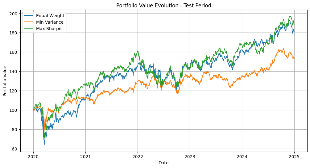
Part 3: Sector-Based Portfolio Analysis
Question 3.1: Creating Sector Returns
Create sector-based returns by averaging returns of stocks within the same sector. First, define sector mappings, then compute their historical returns using our existing returns data.
Hint: - Define a dictionary mapping sectors to their constituent stocks - Use pandas mean() function to compute average returns - Remember to handle the train/test split consistently with previous analysis
# Define sector mappings
sector_mapping = {
    'Technology': ['AAPL', 'MSFT', 'INTC', 'CSCO', 'ORCL'],
    'Financial': ['JPM', 'BAC', 'GS', 'MS', 'C', 'AXP', 'WFC'],
    'Healthcare': ['JNJ', 'PFE', 'MRK', 'ABT', 'BMY'],
    'Energy': ['XOM', 'CVX', 'COP', 'SLB', 'OXY'],
    'Consumer_Staples': ['WMT', 'PG', 'KO', 'PEP', 'CL', 'KMB', 'GIS'],
    'Consumer_Discretionary': ['HD', 'MCD', 'NKE', 'SBUX', 'TJX', 'LOW', 'YUM'],
    'Industrial': ['CAT', 'BA', 'MMM', 'HON', 'GE', 'DE', 'FDX'],
    'Materials': ['APD', 'ECL', 'NEM', 'FCX', 'PPG', 'NUE'],
    'Telecommunications': ['VZ', 'T', 'CMCSA'],
    'Real_Estate': ['SPG', 'PSA']
}


# Calculate sector returns
sector_returns = pd.DataFrame()
for sector, stocks in sector_mapping.items():
    sector_returns[sector] = returns[stocks].mean(axis=1)

# Split into training and testing periods
train_sector_returns = sector_returns[returns.index < split_date]
test_sector_returns = sector_returns[returns.index >= split_date]

# Display summary statistics for training period
print("Sector Returns Summary (Training Period):")
print(train_sector_returns.describe())

# Display correlations between sectors
print("\nSector Return Correlations (Training Period):")
print(train_sector_returns.corr())
Sector Returns Summary (Training Period):
Technology Financial Healthcare Energy Consumer_Staples \
count 2515.000000 2515.000000 2515.000000 2515.000000 2515.000000
mean 0.000708 0.000529 0.000561 0.000228 0.000435
std 0.011622 0.015460 0.009070 0.013255 0.007475
min -0.056637 -0.120743 -0.048842 -0.080151 -0.039052
25% -0.004963 -0.006888 -0.004165 -0.006827 -0.003661
50% 0.000966 0.000601 0.000699 0.000480 0.000543
75% 0.006897 0.008406 0.005836 0.007352 0.004696
max 0.063131 0.090448 0.049754 0.058274 0.035414
Consumer_Discretionary Industrial Materials Telecommunications \
count 2515.000000 2515.000000 2515.000000 2515.000000
mean 0.000850 0.000571 0.000464 0.000605
std 0.009784 0.011905 0.013003 0.009453
min -0.055153 -0.069274 -0.058961 -0.054617
25% -0.004366 -0.005423 -0.006640 -0.004637
50% 0.001120 0.000822 0.000835 0.001034
75% 0.006386 0.006830 0.007747 0.006185
max 0.058083 0.059283 0.075934 0.038374
Real_Estate
count 2515.000000
mean 0.000552
std 0.011736
min -0.079154
25% -0.005862
50% 0.000981
75% 0.007002
max 0.109263
Sector Return Correlations (Training Period):
Technology Financial Healthcare Energy \
Technology 1.000000 0.652064 0.603375 0.597924
Financial 0.652064 1.000000 0.572227 0.634610
Healthcare 0.603375 0.572227 1.000000 0.527469
Energy 0.597924 0.634610 0.527469 1.000000
Consumer_Staples 0.515071 0.434815 0.616829 0.436855
Consumer_Discretionary 0.673522 0.631643 0.607782 0.538476
Industrial 0.739289 0.762015 0.628253 0.719753
Materials 0.619829 0.639049 0.543687 0.716903
Telecommunications 0.553905 0.557995 0.584180 0.523741
Real_Estate 0.473704 0.491617 0.476236 0.440345
Consumer_Staples Consumer_Discretionary Industrial \
Technology 0.515071 0.673522 0.739289
Financial 0.434815 0.631643 0.762015
Healthcare 0.616829 0.607782 0.628253
Energy 0.436855 0.538476 0.719753
Consumer_Staples 1.000000 0.603731 0.535556
Consumer_Discretionary 0.603731 1.000000 0.704662
Industrial 0.535556 0.704662 1.000000
Materials 0.466227 0.579457 0.751812
Telecommunications 0.613324 0.583881 0.610452
Real_Estate 0.532315 0.572199 0.537836
Materials Telecommunications Real_Estate
Technology 0.619829 0.553905 0.473704
Financial 0.639049 0.557995 0.491617
Healthcare 0.543687 0.584180 0.476236
Energy 0.716903 0.523741 0.440345
Consumer_Staples 0.466227 0.613324 0.532315
Consumer_Discretionary 0.579457 0.583881 0.572199
Industrial 0.751812 0.610452 0.537836
Materials 1.000000 0.529148 0.465546
Telecommunications 0.529148 1.000000 0.499715
Real_Estate 0.465546 0.499715 1.000000 Question 3.2: Weight Conversion Function
Create and test a function that converts sector-level portfolio weights into individual stock weights, assuming equal weighting within each sector.
Hint: - Each stock within a sector should have equal weight - The sum of all stock weights should equal 1 - Test the function with simple cases
def sector_to_stock_weights(sector_weights, sector_mapping):
    """
    Convert sector weights to individual stock weights

    Parameters:
    sector_weights: array-like, weights for each sector
    sector_mapping: dict, mapping sectors to stock lists

    Returns:
    dict: Individual stock weights
    """
    stock_weights = {}

    for sector, weight in zip(sector_mapping.keys(), sector_weights):
        stocks_in_sector = sector_mapping[sector]
        weight_per_stock = weight / len(stocks_in_sector)

        for stock in stocks_in_sector:
            stock_weights[stock] = weight_per_stock

    return stock_weights

# Test 1: Equal weights across sectors
print("Test 1: Equal sector weights")
n_sectors = len(sector_mapping)
equal_weights = np.ones(n_sectors) / n_sectors

print("\nSector weights:")
for sector, weight in zip(sector_mapping.keys(), equal_weights):
    print(f"{sector}: {weight:.4f}")

equal_stock_weights = sector_to_stock_weights(equal_weights, sector_mapping)
print("\nResulting stock weights:")
for stock, weight in equal_stock_weights.items():
    print(f"{stock}: {weight:.4f}")

# Test 2: Different sector weights
print("\nTest 2: Custom sector weights")
custom_weights = np.array([0.3, 0.2, 0.2, 0.1, 0.1, 0.1])
print("\nSector weights:")
for sector, weight in zip(sector_mapping.keys(), custom_weights):
    print(f"{sector}: {weight:.4f}")

custom_stock_weights = sector_to_stock_weights(custom_weights, sector_mapping)
print("\nResulting stock weights:")
for stock, weight in custom_stock_weights.items():
    print(f"{stock}: {weight:.4f}")

# Verify weights sum to 1
print(f"\nVerification - sum of weights: {sum(custom_stock_weights.values()):.6f}")
Test 1: Equal sector weights
Sector weights:
Technology: 0.1000
Financial: 0.1000
Healthcare: 0.1000
Energy: 0.1000
Consumer_Staples: 0.1000
Consumer_Discretionary: 0.1000
Industrial: 0.1000
Materials: 0.1000
Telecommunications: 0.1000
Real_Estate: 0.1000
Resulting stock weights:
AAPL: 0.0200
MSFT: 0.0200
INTC: 0.0200
CSCO: 0.0200
ORCL: 0.0200
JPM: 0.0143
BAC: 0.0143
GS: 0.0143
MS: 0.0143
C: 0.0143
AXP: 0.0143
WFC: 0.0143
JNJ: 0.0200
PFE: 0.0200
MRK: 0.0200
ABT: 0.0200
BMY: 0.0200
XOM: 0.0200
CVX: 0.0200
COP: 0.0200
SLB: 0.0200
OXY: 0.0200
WMT: 0.0143
PG: 0.0143
KO: 0.0143
PEP: 0.0143
CL: 0.0143
KMB: 0.0143
GIS: 0.0143
HD: 0.0143
MCD: 0.0143
NKE: 0.0143
SBUX: 0.0143
TJX: 0.0143
LOW: 0.0143
YUM: 0.0143
CAT: 0.0143
BA: 0.0143
MMM: 0.0143
HON: 0.0143
GE: 0.0143
DE: 0.0143
FDX: 0.0143
APD: 0.0167
ECL: 0.0167
NEM: 0.0167
FCX: 0.0167
PPG: 0.0167
NUE: 0.0167
VZ: 0.0333
T: 0.0333
CMCSA: 0.0333
SPG: 0.0500
PSA: 0.0500
Test 2: Custom sector weights
Sector weights:
Technology: 0.3000
Financial: 0.2000
Healthcare: 0.2000
Energy: 0.1000
Consumer_Staples: 0.1000
Consumer_Discretionary: 0.1000
Resulting stock weights:
AAPL: 0.0600
MSFT: 0.0600
INTC: 0.0600
CSCO: 0.0600
ORCL: 0.0600
JPM: 0.0286
BAC: 0.0286
GS: 0.0286
MS: 0.0286
C: 0.0286
AXP: 0.0286
WFC: 0.0286
JNJ: 0.0400
PFE: 0.0400
MRK: 0.0400
ABT: 0.0400
BMY: 0.0400
XOM: 0.0200
CVX: 0.0200
COP: 0.0200
SLB: 0.0200
OXY: 0.0200
WMT: 0.0143
PG: 0.0143
KO: 0.0143
PEP: 0.0143
CL: 0.0143
KMB: 0.0143
GIS: 0.0143
HD: 0.0143
MCD: 0.0143
NKE: 0.0143
SBUX: 0.0143
TJX: 0.0143
LOW: 0.0143
YUM: 0.0143
Verification - sum of weights: 1.000000Question 3.3: Sector Portfolio Optimization
Using the training period data, optimize sector-based portfolios for minimum variance and maximum Sharpe ratio. Compare with an equal-weight sector allocation.
Hint: - Use the same optimization approach as in Part 2 - Remember to create new constraints for the number of sectors - Use only training period data for optimization
# Calculate training period metrics
train_sector_mean_returns = train_sector_returns.mean()
train_sector_cov_matrix = train_sector_returns.cov()

# Define optimization constraints for sectors
n_sectors = len(sector_mapping)
sector_constraints = ({'type': 'eq', 'fun': lambda x: np.sum(x) - 1})
sector_bounds = tuple((0, 1) for _ in range(n_sectors))

# Optimize minimum variance portfolio
sector_min_var_result = minimize(
    lambda w: portfolio_metrics(w, train_sector_mean_returns, train_sector_cov_matrix)[1],
    np.ones(n_sectors)/n_sectors,
    constraints=sector_constraints,
    bounds=sector_bounds,
    method='SLSQP'
)

# Optimize maximum Sharpe ratio portfolio
sector_max_sharpe_result = minimize(
    lambda w: -portfolio_metrics(w, train_sector_mean_returns, train_sector_cov_matrix)[0]/
             portfolio_metrics(w, train_sector_mean_returns, train_sector_cov_matrix)[1],
    np.ones(n_sectors)/n_sectors,
    constraints=sector_constraints,
    bounds=sector_bounds,
    method='SLSQP'
)

# Print optimization results
print("Minimum Variance Portfolio Weights:")
for sector, weight in zip(sector_mapping.keys(), sector_min_var_result.x):
    print(f"{sector}: {weight:.4f}")

print("\nMaximum Sharpe Ratio Portfolio Weights:")
for sector, weight in zip(sector_mapping.keys(), sector_max_sharpe_result.x):
    print(f"{sector}: {weight:.4f}")
Minimum Variance Portfolio Weights:
Technology: 0.0000
Financial: 0.0000
Healthcare: 0.2300
Energy: 0.0000
Consumer_Staples: 0.4999
Consumer_Discretionary: 0.0869
Industrial: 0.0000
Materials: 0.0000
Telecommunications: 0.1832
Real_Estate: 0.0000
Maximum Sharpe Ratio Portfolio Weights:
Technology: 0.0000
Financial: 0.0000
Healthcare: 0.0861
Energy: 0.0000
Consumer_Staples: 0.0000
Consumer_Discretionary: 0.7308
Industrial: 0.0000
Materials: 0.0000
Telecommunications: 0.1831
Real_Estate: 0.0000Question 3.4: Portfolio Visualization
Create visualizations to compare the sector allocations and corresponding stock allocations for each portfolio strategy.
Hint: - Use pie charts to show both sector and stock level allocations - Use the sector_to_stock_weights function from Question 3.2 - Consider using subplots for clear comparison
# Define portfolio strategies
portfolios = {
    'Equal-Weight': np.ones(n_sectors)/n_sectors,
    'Min Variance': sector_min_var_result.x,
    'Max Sharpe': sector_max_sharpe_result.x
}

# Create visualization
plt.figure(figsize=(15, 10))

for idx, (name, weights) in enumerate(portfolios.items(), 1):
    # Sector weights
    plt.subplot(2, 3, idx)
    plt.pie(weights, labels=sector_mapping.keys(), autopct='%1.1f%%')
    plt.title(f'{name}\nSector Allocation')

    # Stock weights
    plt.subplot(2, 3, idx+3)
    stock_weights = sector_to_stock_weights(weights, sector_mapping)
    plt.pie(list(stock_weights.values()),
            labels=list(stock_weights.keys()),
            autopct='%1.1f%%')
    plt.title(f'{name}\nStock Allocation')

plt.tight_layout()
plt.show()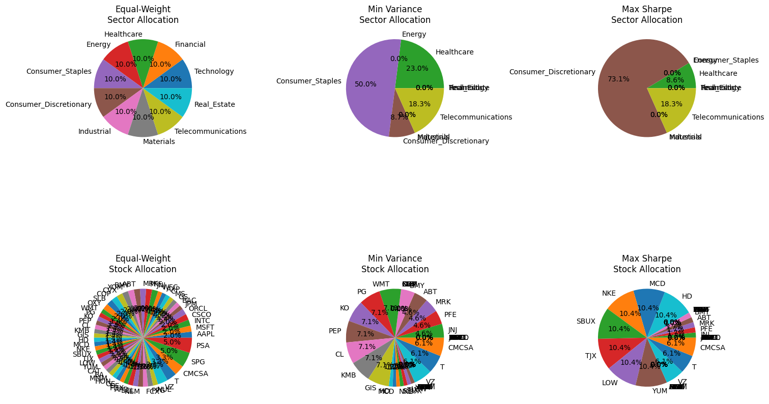
Part 4: Risk Analysis
Question 4.1: Risk Metrics Function
Create a function to calculate various risk metrics for a return series: - Maximum Drawdown - Sortino Ratio - Value at Risk (VaR) - Conditional Value at Risk (CVaR)
Hint: - Use cumulative returns for drawdown calculation - Consider using numpy percentile for VaR - Remember to annualize metrics where appropriate
def calculate_risk_metrics(returns, rf_rate=0.02/252):  # Default daily risk-free rate
    """
    Calculate various risk metrics for a return series

    Parameters:
    returns: Series of returns
    rf_rate: Daily risk-free rate

    Returns:
    dict: Dictionary of risk metrics
    """
    # Maximum Drawdown
    cum_returns = (1 + returns).cumprod()
    running_max = cum_returns.cummax()
    drawdowns = (cum_returns - running_max) / running_max
    max_drawdown = drawdowns.min()

    # Sortino Ratio
    excess_returns = returns - rf_rate
    downside_returns = returns[returns < 0]
    downside_std = np.std(downside_returns, ddof=1)
    sortino = np.sqrt(252) * excess_returns.mean() / downside_std

    # Value at Risk (95%)
    var_95 = np.percentile(returns, 5)

    # Conditional Value at Risk (Expected Shortfall)
    cvar_95 = returns[returns <= var_95].mean()

    return {
        'Maximum Drawdown': max_drawdown,
        'Sortino Ratio': sortino,
        'VaR (95%)': var_95,
        'CVaR (95%)': cvar_95
    }

# Test the function on training data
print("Risk Metrics for Equal-Weight Sector Portfolio (Training Period):")
equal_weight_returns = train_sector_returns @ (np.ones(n_sectors)/n_sectors)
metrics = calculate_risk_metrics(equal_weight_returns)
for metric, value in metrics.items():
    print(f"{metric}: {value:.4f}")
Risk Metrics for Equal-Weight Sector Portfolio (Training Period):
Maximum Drawdown: -0.1618
Sortino Ratio: 1.0901
VaR (95%): -0.0144
CVaR (95%): -0.0216Question 4.2: CAPM Analysis
Calculate CAPM metrics (alpha and beta) for sector portfolios. Compare the risk-adjusted performance across different portfolio strategies.
Hint: - Download market data (S&P 500) for the same period - Use linear regression to calculate beta - Remember to annualize alpha
import statsmodels.api as sm

# Download market data
market_data = yf.download('^GSPC', start=start_date, end=end_date)['Close']
market_returns = market_data.pct_change().dropna()

def calculate_capm_metrics(returns, market_returns, rf_rate=0.02/252):
    """
    Calculate CAPM metrics

    Returns:
    tuple: (alpha, beta)
    """
    # Prepare data for regression
    excess_returns = returns - rf_rate
    excess_market_returns = market_returns - rf_rate

    # Add constant for regression
    X = sm.add_constant(excess_market_returns)

    # Perform regression
    model = sm.OLS(excess_returns, X).fit()

    # Extract and annualize alpha
    alpha = model.params[0] * 252
    beta = model.params[1]

    return alpha, beta

# Calculate CAPM metrics for each portfolio
for name, weights in portfolios.items():
    print(f"\n{name} Portfolio CAPM Metrics:")

    # Training period
    portfolio_returns = train_sector_returns @ weights
    train_market_returns = market_returns[market_returns.index < split_date]
    alpha, beta = calculate_capm_metrics(portfolio_returns, train_market_returns)
    print(f"Training Period - Alpha: {alpha:.4%}, Beta: {beta:.4f}")

    # Testing period
    portfolio_returns = test_sector_returns @ weights
    test_market_returns = market_returns[market_returns.index >= split_date]
    alpha, beta = calculate_capm_metrics(portfolio_returns, test_market_returns)
    print(f"Testing Period - Alpha: {alpha:.4%}, Beta: {beta:.4f}")
[*********************100%***********************] 1 of 1 completed
/var/folders/dr/3gd86y8j4w19p8jdnqy5s65m0000gp/T/ipykernel_70455/2328182781.py:25: FutureWarning: Series.__getitem__ treating keys as positions is deprecated. In a future version, integer keys will always be treated as labels (consistent with DataFrame behavior). To access a value by position, use `ser.iloc[pos]`
alpha = model.params[0] * 252
/var/folders/dr/3gd86y8j4w19p8jdnqy5s65m0000gp/T/ipykernel_70455/2328182781.py:26: FutureWarning: Series.__getitem__ treating keys as positions is deprecated. In a future version, integer keys will always be treated as labels (consistent with DataFrame behavior). To access a value by position, use `ser.iloc[pos]`
beta = model.params[1]
Equal-Weight Portfolio CAPM Metrics:
Training Period - Alpha: 2.8582%, Beta: 0.9390
Testing Period - Alpha: 0.6888%, Beta: 0.9013

Min Variance Portfolio CAPM Metrics:
Training Period - Alpha: 5.2233%, Beta: 0.6415
Testing Period - Alpha: -1.0409%, Beta: 0.5726

Max Sharpe Portfolio CAPM Metrics:
Training Period - Alpha: 9.7843%, Beta: 0.8203
Testing Period - Alpha: -1.7344%, Beta: 0.8535
Question 4.3: Performance Comparison
Compare the performance of sector-based portfolios with the individual stock portfolios from Part 2. Create visualizations showing the cumulative returns and risk metrics for both approaches.
Hint: - Use the optimal portfolios from both Parts 2 and 3 - Plot cumulative returns on the same graph - Create a summary table of risk metrics
# Calculate cumulative returns for all portfolios
plt.figure(figsize=(12, 6))

# Plot sector portfolios
for name, weights in portfolios.items():
    portfolio_returns = pd.concat([
        train_sector_returns @ weights,
        test_sector_returns @ weights
    ])
    cum_returns = (1 + portfolio_returns).cumprod()
    plt.plot(cum_returns.index, cum_returns,
             label=f'Sector {name}', linestyle='-')

# Plot individual stock portfolios from Part 2
individual_portfolios = {
    'Min Variance': min_var_result.x,
    'Max Sharpe': max_sharpe_result.x
}

for name, weights in individual_portfolios.items():
    portfolio_returns = returns @ weights
    cum_returns = (1 + portfolio_returns).cumprod()
    plt.plot(cum_returns.index, cum_returns,
             label=f'Stock {name}', linestyle='--')

plt.axvline(x=pd.to_datetime(split_date), color='black',
            linestyle=':', label='Train/Test Split')
plt.title('Cumulative Returns Comparison')
plt.xlabel('Date')
plt.ylabel('Cumulative Return')
plt.legend()
plt.grid(True)
plt.show()

# Compare risk metrics
print("\nRisk Metrics Comparison (Testing Period):")
all_portfolios = {
    'Sector Equal-Weight': np.ones(n_sectors)/n_sectors,
    'Sector Min Variance': sector_min_var_result.x,
    'Sector Max Sharpe': sector_max_sharpe_result.x,
    'Stock Min Variance': min_var_result.x,
    'Stock Max Sharpe': max_sharpe_result.x
}

for name, weights in all_portfolios.items():
    print(f"\n{name}:")
    if 'Sector' in name:
        returns_series = test_sector_returns @ weights
    else:
        returns_series = test_returns @ weights

    metrics = calculate_risk_metrics(returns_series)
    for metric, value in metrics.items():
        print(f"{metric}: {value:.4f}")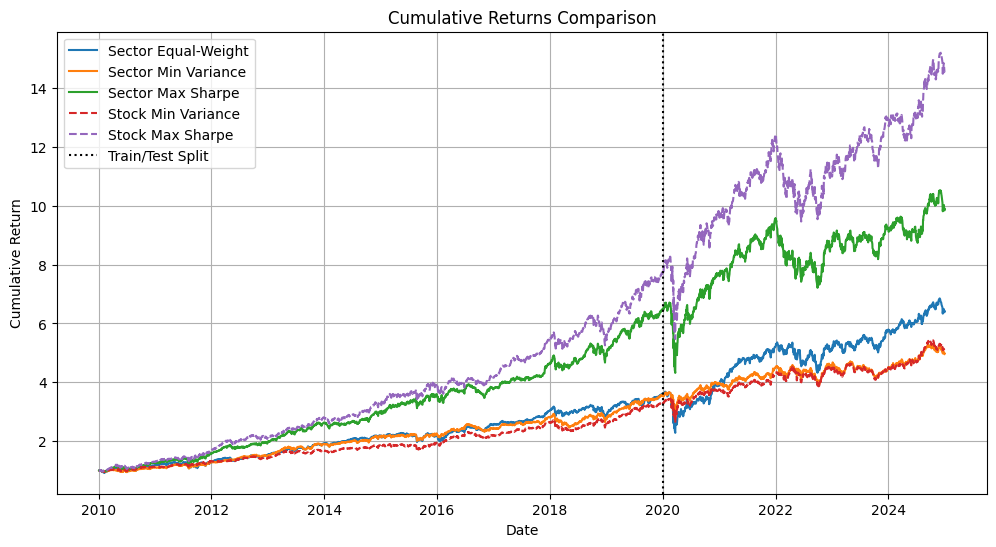
Risk Metrics Comparison (Testing Period):

Sector Equal-Weight:
Maximum Drawdown: -0.3801
Sortino Ratio: 0.6716
VaR (95%): -0.0170
CVaR (95%): -0.0311

Sector Min Variance:
Maximum Drawdown: -0.2407
Sortino Ratio: 0.4855
VaR (95%): -0.0136
CVaR (95%): -0.0229

Sector Max Sharpe:
Maximum Drawdown: -0.3563
Sortino Ratio: 0.5206
VaR (95%): -0.0174
CVaR (95%): -0.0301

Stock Min Variance:
Maximum Drawdown: -0.2395
Sortino Ratio: 0.6236
VaR (95%): -0.0134
CVaR (95%): -0.0226

Stock Max Sharpe:
Maximum Drawdown: -0.3405
Sortino Ratio: 0.7347
VaR (95%): -0.0177
CVaR (95%): -0.0309
# Calculate cumulative returns for all portfolios
plt.figure(figsize=(12, 6))
# Plot sector portfolios
for name, weights in portfolios.items():
portfolio_returns = test_sector_returns @ weights
cum_returns = (1 + portfolio_returns).cumprod()
plt.plot(cum_returns.index, cum_returns,
label=f'Sector {name}', linestyle='-')
# Plot individual stock portfolios from Part 2
individual_portfolios = {
'Min Variance': min_var_result.x,
'Max Sharpe': max_sharpe_result.x
}
for name, weights in individual_portfolios.items():
portfolio_returns = test_returns @ weights
cum_returns = (1 + portfolio_returns).cumprod()
plt.plot(cum_returns.index, cum_returns,
label=f'Stock {name}', linestyle='--')
plt.axvline(x=pd.to_datetime(split_date), color='black',
linestyle=':', label='Train/Test Split')
plt.title('Cumulative Returns Comparison')
plt.xlabel('Date')
plt.ylabel('Cumulative Return')
plt.legend()
plt.grid(True)
plt.show()
# Compare risk metrics
print("\nRisk Metrics Comparison (Testing Period):")
all_portfolios = {
'Sector Equal-Weight': np.ones(n_sectors)/n_sectors,
'Sector Min Variance': sector_min_var_result.x,
'Sector Max Sharpe': sector_max_sharpe_result.x,
'Stock Min Variance': min_var_result.x,
'Stock Max Sharpe': max_sharpe_result.x
}
for name, weights in all_portfolios.items():
print(f"\n{name}:")
if 'Sector' in name:
returns_series = test_sector_returns @ weights
else:
returns_series = test_returns @ weights
metrics = calculate_risk_metrics(returns_series)
for metric, value in metrics.items():
print(f"{metric}: {value:.4f}")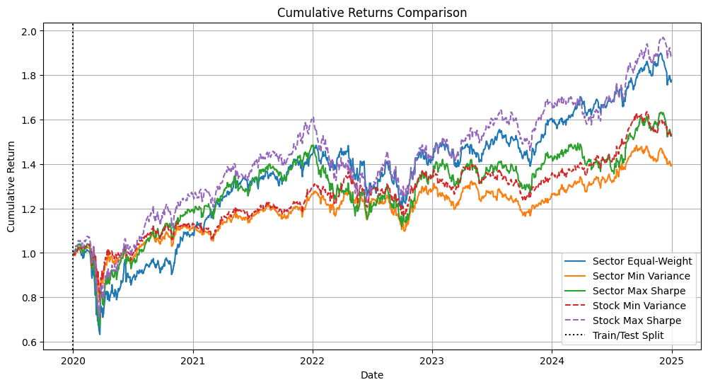
Risk Metrics Comparison (Testing Period):

Sector Equal-Weight:
Maximum Drawdown: -0.3801
Sortino Ratio: 0.6716
VaR (95%): -0.0170
CVaR (95%): -0.0311

Sector Min Variance:
Maximum Drawdown: -0.2407
Sortino Ratio: 0.4855
VaR (95%): -0.0136
CVaR (95%): -0.0229

Sector Max Sharpe:
Maximum Drawdown: -0.3563
Sortino Ratio: 0.5206
VaR (95%): -0.0174
CVaR (95%): -0.0301

Stock Min Variance:
Maximum Drawdown: -0.2395
Sortino Ratio: 0.6236
VaR (95%): -0.0134
CVaR (95%): -0.0226

Stock Max Sharpe:
Maximum Drawdown: -0.3405
Sortino Ratio: 0.7347
VaR (95%): -0.0177
CVaR (95%): -0.0309