TP Python for Finance: Introduction to Option Pricing
Author
Remi Genet
Published
2025-02-12
Question 1: Data Collection
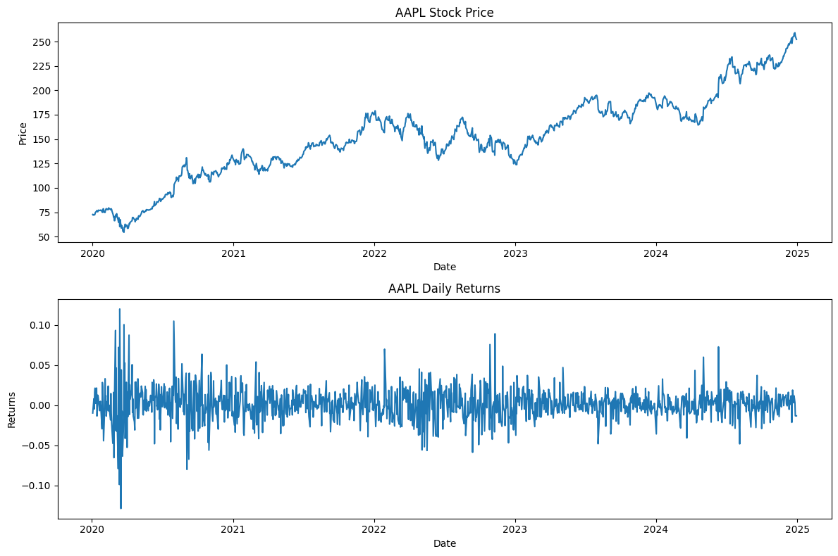
Using the yfinance library, download daily price data for the stock “AAPL” (Apple Inc.) for the last year. Calculate and plot the daily returns of the stock.
import yfinance as yfimport pandas as pdimport numpy as npimport matplotlib.pyplot as plt# Download the dataticker ="AAPL"start_date ="2020-01-01"end_date ="2024-12-31"# Your code here to:# 1. Download the data using yfinance# 2. Calculate daily returns# 3. Create a plot of the stock price and returns
[*********************100%***********************] 1 of 1 completed
Question 2: Understanding Call Options
A Call option is a financial contract that gives the buyer the right (but not the obligation) to buy a stock at a predetermined price (strike price) at a future date (expiration date). The seller of the option (writer) receives a premium for taking on the obligation to sell at the strike price if the buyer exercises their right.
Example: If you buy a call option for AAPL with: - Strike price (K) = $180 - Current price (S) = $170 - Expiration = 1 month
If at expiration: - AAPL price = $190: Your profit = $190 - $180 = $10 (minus the premium paid) - AAPL price = $170: Your loss = premium paid
Create a function that calculates the payoff of a call option at expiration.
# Your code here to:# Create a function that takes as input:# - Strike price (K)# - Current price (S)# And returns the payoff at expiration
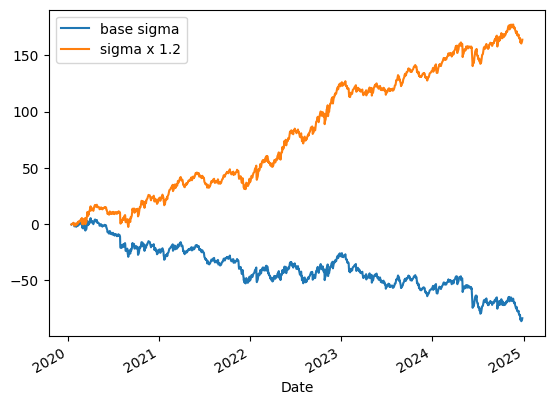
Create a function that simulates future stock prices using Monte Carlo simulation. We’ll use the following assumptions: - Stock returns are normally distributed (Note: This is a simplifying assumption that doesn’t hold well in reality) - The volatility is estimated from historical data
# Your code here to:# 1. Create a function that simulates stock paths# 2. Use it to estimate option prices
Estimated call option price: 0.81
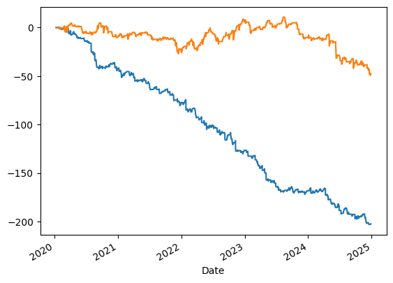
Question 4: Competing Option Sellers
Two option sellers are competing in the market. They use different methods to estimate volatility: - Seller 1: Uses 5-day rolling standard deviation - Seller 2: Uses 10-day rolling standard deviation
Follow these steps to simulate their competition:
First, calculate the rolling volatility for each seller:
Use rolling() function with window=5 for seller 1
Use rolling() function with window=10 for seller 2
Don’t forget to use .std() to get the standard deviation
For each day, calculate the option price that each seller would offer:
Use the estimate_call_price function we created earlier
You can use apply() with a lambda function to calculate prices
Each seller uses their own volatility estimate
Determine which seller makes the sale:
The seller with the lower price wins the trade
Use comparison operators and astype(int) to create indicator variables