The Multi-Layer Perceptron (MLP)

The MLP is the fundamental building block of deep learning. This chapter breaks down its biological inspiration, mathematical formulation, and financial applications.

The Building Block: MLP Architecture

---

Section 1.6 - From Biological Neurons to Artificial Networks

Inspiration

MLPs are loosely inspired by how biological neurons process information:

• Dendrites: Receive inputs like the feature vector \[ \mathbf{x} \]
• Cell body: Aggregates signals by computing the weighted sum \[ \mathbf{w}^\top \mathbf{x} + b \]
• Axon: Transmits the output through synapses via the activation function \[ \varphi \]

MLP Structure

---

Section 1.7 - Mathematical Formulation

Single Neuron (Perceptron)

For an input vector \[ \mathbf{x} \in \mathbb{R}^d, \] the computation is as follows:

Computation:
\[ z = \mathbf{w}^\top \mathbf{x} + b, \] \[ a = \varphi(z). \]

Where: - \[\mathbf{w} \in \mathbb{R}^d\] is the weight vector (learnable) - \[b \in \mathbb{R}\] is the bias term (learnable) - \[\varphi\] is the non-linear activation function

Full MLP Layer

A layer with ( n ) neurons produces an output vector \[ \mathbf{a} \in \mathbb{R}^n: \]

Matrix Form:
\[ \mathbf{a} = \varphi(\mathbf{W}\mathbf{x} + \mathbf{b}), \]

Where: - \[\mathbf{W} \in \mathbb{R}^{n \times d}\] is the weight matrix - \[\mathbf{b} \in \mathbb{R}^n\] is the bias vector

---

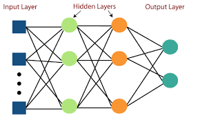
Section 1.8 - Layered Composition

Key Components

1. Input Layer: Raw features (e.g., financial ratios, price returns)
2. Hidden Layers: Successive transformations
   \[ \mathbf{h}^{(l)} = \varphi\left(\mathbf{W}^{(l)}\mathbf{h}^{(l-1)} + \mathbf{b}^{(l)}\right) \]
3. Output Layer: Task-specific format
   • Regression: Uses a linear activation (e.g., to predict stock price)
   • Classification: Uses softmax (e.g., to generate buy/hold/sell signals)

---

Section 1.9 - Activation Functions

Function	Formula	Financial Use Case
ReLU	\[\max(0, z)\]	Default for hidden layers
Sigmoid	\[\frac{1}{1+e^{-z}}\]	Probability outputs (0-1)
Tanh	\[\frac{e^z - e^{-z}}{e^z + e^{-z}}\]	Normalized outputs (-1 to 1)
Linear	\[z\]	Final layer for regression

---

Section 1.10 - Why Hierarchical Layers Matter

Financial Feature Learning

• Layer 1: Extracts simple patterns
  (e.g., momentum, mean reversion)
• Layer 2: Combines patterns
  (e.g., momentum + volatility regime)
• Layer 3: Leads to a strategic decision
  (e.g., optimal portfolio weight)

Example:
Raw Input → Volatility Estimates → Regime Detection → Trade Signal

---

Section 1.11 - Code Sketch (Keras)

from keras import layers, models

# Simple MLP for return prediction
model = models.Sequential([
    layers.Dense(32, activation='relu', input_shape=(num_features,)),
    layers.Dense(16, activation='tanh'),
    layers.Dense(1)  # Linear activation for regression
])

---

Historical Note

MLPs gained prominence in the 1980s-90s for: - Stock price prediction (White, 1988) - Credit scoring (Altman et al., 1994)

However, they were limited by computational power until the resurgence of deep learning in the 2010s.

---