DeepLearning For Finance
  • Back to Main Website
  • Home
  • Introduction to Deep Learning
    • Introduction to Deep Learning
    • From Traditional Models to Deep Learning
    • The Multi-Layer Perceptron (MLP)
    • Automatic Differentiation: The Engine of Deep Learning
    • Computation Backends & Keras 3
    • GPUs and Deep Learning: When Hardware Matters
    • Keras Fundamentals: Models & Layers
    • Keras Matrix Operations: The Building Blocks
    • Activation Functions: Adding Non-linearity
    • Model Training Fundamentals

    • Travaux Pratiques
    • TP1 Corrected: Building Neural Networks - From Simple to Custom Implementations
    • TP1 Corrected: Building Neural Networks - From Simple to Custom Implementations
  • Recurrent Neural Networks
    • Recurrent Neural Networks
    • Sequential Data Processing: From MLPs to RNNs
    • Long Short-Term Memory Networks (LSTM)
    • Modern RNN Architectures
    • RNN Limitations: Computational Challenges

    • Travaux Pratiques
    • TP: Recurrent Neural Networks for Time Series Prediction
    • TP Corrected: Recurrent Neural Networks for Time Series Prediction
  • Training a Neural Network
    • Training a Neural Network
    • Understanding the Training Loop
    • Understanding Optimizers
    • Understanding Callbacks
    • Training Parameters and Practical Considerations

    • Travaux Pratiques
    • TP: Using Deep Learning Frameworks for General Optimization
    • tp_general_optimization_corrected.html
    • TP: Impact of Callbacks on Training
  • Essential Building Blocks of Modern Neural Networks
    • Essential Building Blocks of Modern Neural Networks
    • Residual Connections and Gating Mechanisms
    • Convolutional Layers: From Images to Time Series
    • Neural Network Embeddings: Learning Meaningful Representations
    • Attention Mechanisms: Learning What to Focus On
    • Encoder-Decoder Architectures

    • Travaux Pratiques
    • Practical Assignment: Building a Transformer-Based Architecture for Time Series Forecasting
    • Practical Assignment: Building a Transformer-Based Architecture for Time Series Forecasting
  • Projets
    • Projets
  • Code source
  1. Travaux Pratiques
  2. tp_general_optimization_corrected.html
  • Training a Neural Network
  • Understanding the Training Loop
  • Understanding Optimizers
  • Understanding Callbacks
  • Training Parameters and Practical Considerations
  • Travaux Pratiques
    • TP: Using Deep Learning Frameworks for General Optimization
    • tp_general_optimization_corrected.html
    • TP: Impact of Callbacks on Training
    • content/Cours_3/keras_callbacks_corrected.ipynb
  1. Travaux Pratiques
  2. tp_general_optimization_corrected.html
Author

Remi Genet

Published

2025-04-03

import numpy as np
import jax
import jax.numpy as jnp
from jax import grad, jit
from jax.example_libraries import optimizers  # for Adam optimizer
from scipy.optimize import minimize
import time
from functools import partial
import pandas as pd
import matplotlib.pyplot as plt
from typing import Tuple
from dataclasses import dataclass

# Set random seed for reproducibility
np.random.seed(42)
jax.config.update("jax_enable_x64", True)

@dataclass
class EarlyStoppingState:
    """State for early stopping and learning rate scheduling."""
    best_sharpe: float = float('-inf')
    patience_counter: int = 0
    best_weights: jnp.ndarray = None
    lr: float = 0.1
    plateau_counter: int = 0

def generate_data(n_assets: int) -> Tuple[np.ndarray, np.ndarray]:
    """Generate random correlation matrix and expected returns."""
    A = np.random.randn(n_assets, n_assets)
    corr = A @ A.T
    corr = corr / np.max(np.abs(corr))
    returns = np.random.randn(n_assets) * 0.1 + 0.05
    return corr, returns

# SciPy Implementation remains the same as before
def portfolio_stats_scipy(weights: np.ndarray, 
                         corr: np.ndarray, 
                         returns: np.ndarray, 
                         risk_free_rate: float = 0.02) -> Tuple[float, float, float]:
    port_return = np.sum(returns * weights)
    port_vol = np.sqrt(weights.T @ corr @ weights)
    sharpe = (port_return - risk_free_rate) / port_vol
    return port_return, port_vol, sharpe

def negative_sharpe_scipy(weights: np.ndarray, 
                         corr: np.ndarray, 
                         returns: np.ndarray, 
                         risk_free_rate: float = 0.02) -> float:
    _, _, sharpe = portfolio_stats_scipy(weights, corr, returns, risk_free_rate)
    return -sharpe

def optimize_scipy(corr: np.ndarray, returns: np.ndarray) -> Tuple[np.ndarray, float, float]:
    n_assets = len(returns)
    constraints = ({'type': 'eq', 'fun': lambda x: np.sum(x) - 1})
    bounds = tuple((0, 1) for _ in range(n_assets))
    
    start_time = time.time()
    x0 = np.ones(n_assets) / n_assets
    
    result = minimize(negative_sharpe_scipy, x0,
                     args=(corr, returns),
                     method='SLSQP',
                     bounds=bounds,
                     constraints=constraints)
    
    end_time = time.time()
    print('scipy optimization succeed:', result.success)
    return result.x, -result.fun, end_time - start_time

# JAX Implementation with Adam
@jit
def portfolio_stats_jax(weights: jnp.ndarray, 
                       corr: jnp.ndarray, 
                       returns: jnp.ndarray, 
                       risk_free_rate: float = 0.02) -> Tuple[float, float, float]:
    port_return = jnp.sum(returns * weights)
    port_vol = jnp.sqrt(weights.T @ corr @ weights)
    sharpe = (port_return - risk_free_rate) / port_vol
    return port_return, port_vol, sharpe

@jit
def negative_sharpe_jax(weights: jnp.ndarray, 
                       corr: jnp.ndarray, 
                       returns: jnp.ndarray, 
                       risk_free_rate: float = 0.02) -> float:
    _, _, sharpe = portfolio_stats_jax(weights, corr, returns, risk_free_rate)
    return -sharpe

@jit
def projection_simplex(x: jnp.ndarray) -> jnp.ndarray:
    """Project onto probability simplex."""
    x = jnp.clip(x, 0, None)
    return x / jnp.sum(x)

def update_early_stopping_state(state: EarlyStoppingState, 
                              current_sharpe: float, 
                              current_weights: jnp.ndarray,
                              patience: int = 10,
                              min_improvement: float = 1e-4,
                              lr_reduction_factor: float = 0.5,
                              lr_patience: int = 5,
                              min_lr: float = 1e-6) -> EarlyStoppingState:
    if current_sharpe > state.best_sharpe + min_improvement:
        state.best_sharpe = current_sharpe
        state.best_weights = current_weights
        state.patience_counter = 0
        state.plateau_counter = 0
    else:
        state.patience_counter += 1
        state.plateau_counter += 1
        
        if state.plateau_counter >= lr_patience and state.lr > min_lr:
            state.lr *= lr_reduction_factor
            state.lr = max(state.lr, min_lr)
            state.plateau_counter = 0
            print(f"Reducing learning rate to {state.lr}")
    
    return state

def optimize_jax(corr: np.ndarray, 
                returns: np.ndarray, 
                n_iterations: int = 1000,
                initial_lr: float = 0.01,  # Lower initial learning rate for Adam
                patience: int = 10,
                min_improvement: float = 1e-4,
                lr_patience: int = 5,
                lr_reduction_factor: float = 0.5,
                min_lr: float = 1e-6,
                b1: float = 0.9,  # Adam beta1
                b2: float = 0.999,  # Adam beta2
                eps: float = 1e-8  # Adam epsilon
                ) -> Tuple[np.ndarray, float, float]:
    """Optimize portfolio using JAX with Adam optimizer."""
    # Convert inputs to JAX arrays
    corr = jnp.array(corr)
    returns = jnp.array(returns)
    
    # Initialize weights and early stopping state
    n_assets = len(returns)
    init_weights = jnp.ones(n_assets) / n_assets
    state = EarlyStoppingState(lr=initial_lr, best_weights=init_weights)
    
    start_time = time.time()
    
    # Initialize Adam optimizer
    opt_init, opt_update, get_params = optimizers.adam(
        step_size=state.lr,
        b1=b1,
        b2=b2,
        eps=eps
    )
    opt_state = opt_init(init_weights)
    
    # Gradient function
    grad_sharpe = jit(grad(negative_sharpe_jax))
    
    # Optimization loop
    for iteration in range(n_iterations):
        weights = get_params(opt_state)
        weights = projection_simplex(weights)  # Project to satisfy constraints
        
        gradient = grad_sharpe(weights, corr, returns)
        opt_state = opt_update(iteration, gradient, opt_state)
        
        current_sharpe = -negative_sharpe_jax(weights, corr, returns)
        
        # Update early stopping state
        state = update_early_stopping_state(
            state, 
            current_sharpe, 
            weights,
            patience=patience,
            min_improvement=min_improvement,
            lr_patience=lr_patience,
            lr_reduction_factor=lr_reduction_factor,
            min_lr=min_lr
        )
        
        # Check early stopping condition
        if state.patience_counter >= patience:
            print(f"Early stopping triggered at iteration {iteration}")
            break
    
    end_time = time.time()
    final_sharpe = state.best_sharpe
    
    return np.array(state.best_weights), float(final_sharpe), end_time - start_time

def compare_optimizers() -> pd.DataFrame:
    """Compare JAX and SciPy optimizers using logspaced number of assets."""
    # Create logspaced array of asset numbers from 5 to 500 with 10 points
    asset_numbers = np.unique(np.logspace(np.log10(5), np.log10(500), 10).astype(int))
    results = []
    
    for n_assets in asset_numbers:
        print(f"Processing {n_assets} assets...")
        corr, returns = generate_data(n_assets)
        
        # Run SciPy optimization
        scipy_weights, scipy_sharpe, scipy_time = optimize_scipy(corr, returns)
        
        # Run JAX optimization with Adam
        jax_weights, jax_sharpe, jax_time = optimize_jax(
            corr, 
            returns,
            n_iterations=1000,
            initial_lr=0.01,
            patience=10,
            min_improvement=1e-4,
            lr_patience=5,
            lr_reduction_factor=0.5,
            min_lr=1e-6
        )
        
        results.append({
            'n_assets': n_assets,
            'scipy_time': scipy_time,
            'jax_time': jax_time,
            'scipy_sharpe': scipy_sharpe,
            'jax_sharpe': jax_sharpe
        })
    
    return pd.DataFrame(results)

# Run comparison
results_df = compare_optimizers()

# Create visualization
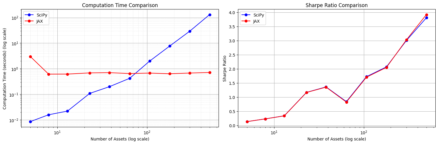
fig, (ax1, ax2) = plt.subplots(1, 2, figsize=(15, 5))

# Plot computation time comparison with log scale
ax1.loglog(results_df['n_assets'], results_df['scipy_time'], 'b-o', label='SciPy')
ax1.loglog(results_df['n_assets'], results_df['jax_time'], 'r-o', label='JAX')
ax1.set_xlabel('Number of Assets (log scale)')
ax1.set_ylabel('Computation Time (seconds) (log scale)')
ax1.set_title('Computation Time Comparison')
ax1.legend()
ax1.grid(True, which="both", ls="-")
ax1.grid(True, which="minor", ls=":", alpha=0.4)


# Plot Sharpe ratio comparison with log scale
ax2.semilogx(results_df['n_assets'], results_df['scipy_sharpe'], 'b-o', label='SciPy')
ax2.semilogx(results_df['n_assets'], results_df['jax_sharpe'], 'r-o', label='JAX')
ax2.set_xlabel('Number of Assets (log scale)')
ax2.set_ylabel('Sharpe Ratio')
ax2.set_title('Sharpe Ratio Comparison')
ax2.legend()
ax2.grid(True)

plt.tight_layout()
print("Results DataFrame:")
print(results_df)
print("\nAsset numbers tested:", sorted(results_df['n_assets'].unique()))
An NVIDIA GPU may be present on this machine, but a CUDA-enabled jaxlib is not installed. Falling back to cpu.
Processing 5 assets...
scipy optimization succeed: True
Reducing learning rate to 0.005
Reducing learning rate to 0.0025
Reducing learning rate to 0.00125
Early stopping triggered at iteration 65
Processing 8 assets...
scipy optimization succeed: True
Reducing learning rate to 0.005
Reducing learning rate to 0.0025
Early stopping triggered at iteration 46
Processing 13 assets...
scipy optimization succeed: True
Reducing learning rate to 0.005
Reducing learning rate to 0.0025
Early stopping triggered at iteration 55
Processing 23 assets...
scipy optimization succeed: True
Reducing learning rate to 0.005
Reducing learning rate to 0.0025
Early stopping triggered at iteration 40
Processing 38 assets...
scipy optimization succeed: True
Reducing learning rate to 0.005
Reducing learning rate to 0.0025
Early stopping triggered at iteration 50
Processing 64 assets...
scipy optimization succeed: True
Reducing learning rate to 0.005
Reducing learning rate to 0.0025
Early stopping triggered at iteration 46
Processing 107 assets...
scipy optimization succeed: True
Reducing learning rate to 0.005
Reducing learning rate to 0.0025
Early stopping triggered at iteration 36
Processing 179 assets...
scipy optimization succeed: False
Reducing learning rate to 0.005
Reducing learning rate to 0.0025
Reducing learning rate to 0.00125
Early stopping triggered at iteration 54
Processing 299 assets...
scipy optimization succeed: False
Reducing learning rate to 0.005
Reducing learning rate to 0.0025
Early stopping triggered at iteration 56
Processing 499 assets...
scipy optimization succeed: False
Reducing learning rate to 0.005
Reducing learning rate to 0.0025
Reducing learning rate to 0.00125
Early stopping triggered at iteration 48
Results DataFrame:
   n_assets  scipy_time  jax_time  scipy_sharpe  jax_sharpe
0         5    0.008611  3.009516      0.135780    0.135646
1         8    0.015914  0.616226      0.232291    0.232144
2        13    0.022206  0.619008      0.341706    0.338631
3        23    0.108918  0.688017      1.169611    1.165775
4        38    0.198324  0.702203      1.361956    1.353065
5        64    0.421465  0.649472      0.842560    0.825843
6       107    1.987418  0.676356      1.723101    1.703693
7       179    7.689285  0.636931      2.070086    2.051470
8       299   29.139531  0.678314      3.003464    3.026304
9       499  130.346113  0.713434      3.805702    3.918855

Asset numbers tested: [np.int64(5), np.int64(8), np.int64(13), np.int64(23), np.int64(38), np.int64(64), np.int64(107), np.int64(179), np.int64(299), np.int64(499)]

Back to top
TP: Using Deep Learning Frameworks for General Optimization
TP: Impact of Callbacks on Training

Deep Learning For Finance, Rémi Genet.
Licence
Code source disponible sur Github


Site construit avec et Quarto
Inspiration pour la mise en forme du site ici
Code source disponible sur GitHub