TP1 Corrected: Building Neural Networks - From Simple to Custom Implementations

!pip install numpy keras jax matplotlib scikit-learn

Requirement already satisfied: numpy in /usr/local/lib/python3.10/dist-packages (2.2.2)
Requirement already satisfied: keras in /usr/local/lib/python3.10/dist-packages (3.8.0)
Requirement already satisfied: jax in /usr/local/lib/python3.10/dist-packages (0.5.0)
Requirement already satisfied: matplotlib in /usr/local/lib/python3.10/dist-packages (3.10.0)
Requirement already satisfied: scikit-learn in /usr/local/lib/python3.10/dist-packages (1.6.1)
Requirement already satisfied: packaging in /usr/local/lib/python3.10/dist-packages (from keras) (24.2)
Requirement already satisfied: ml-dtypes in /usr/local/lib/python3.10/dist-packages (from keras) (0.5.1)
Requirement already satisfied: namex in /usr/local/lib/python3.10/dist-packages (from keras) (0.0.8)
Requirement already satisfied: rich in /usr/local/lib/python3.10/dist-packages (from keras) (13.9.4)
Requirement already satisfied: optree in /usr/local/lib/python3.10/dist-packages (from keras) (0.14.0)
Requirement already satisfied: h5py in /usr/local/lib/python3.10/dist-packages (from keras) (3.12.1)
Requirement already satisfied: absl-py in /usr/local/lib/python3.10/dist-packages (from keras) (2.1.0)
Requirement already satisfied: opt_einsum in /usr/local/lib/python3.10/dist-packages (from jax) (3.4.0)
Requirement already satisfied: jaxlib<=0.5.0,>=0.5.0 in /usr/local/lib/python3.10/dist-packages (from jax) (0.5.0)
Requirement already satisfied: scipy>=1.11.1 in /usr/local/lib/python3.10/dist-packages (from jax) (1.15.1)
Requirement already satisfied: contourpy>=1.0.1 in /usr/local/lib/python3.10/dist-packages (from matplotlib) (1.3.1)
Requirement already satisfied: fonttools>=4.22.0 in /usr/local/lib/python3.10/dist-packages (from matplotlib) (4.55.8)
Requirement already satisfied: kiwisolver>=1.3.1 in /usr/local/lib/python3.10/dist-packages (from matplotlib) (1.4.8)
Requirement already satisfied: pyparsing>=2.3.1 in /usr/lib/python3/dist-packages (from matplotlib) (2.4.7)
Requirement already satisfied: cycler>=0.10 in /usr/local/lib/python3.10/dist-packages (from matplotlib) (0.12.1)
Requirement already satisfied: pillow>=8 in /usr/local/lib/python3.10/dist-packages (from matplotlib) (11.1.0)
Requirement already satisfied: python-dateutil>=2.7 in /usr/local/lib/python3.10/dist-packages (from matplotlib) (2.9.0.post0)
Requirement already satisfied: threadpoolctl>=3.1.0 in /usr/local/lib/python3.10/dist-packages (from scikit-learn) (3.5.0)
Requirement already satisfied: joblib>=1.2.0 in /usr/local/lib/python3.10/dist-packages (from scikit-learn) (1.4.2)
Requirement already satisfied: six>=1.5 in /usr/lib/python3/dist-packages (from python-dateutil>=2.7->matplotlib) (1.16.0)
Requirement already satisfied: typing-extensions>=4.5.0 in /usr/local/lib/python3.10/dist-packages (from optree->keras) (4.12.2)
Requirement already satisfied: pygments<3.0.0,>=2.13.0 in /usr/local/lib/python3.10/dist-packages (from rich->keras) (2.19.1)
Requirement already satisfied: markdown-it-py>=2.2.0 in /usr/local/lib/python3.10/dist-packages (from rich->keras) (3.0.0)
Requirement already satisfied: mdurl~=0.1 in /usr/local/lib/python3.10/dist-packages (from markdown-it-py>=2.2.0->rich->keras) (0.1.2)
WARNING: Running pip as the 'root' user can result in broken permissions and conflicting behaviour with the system package manager. It is recommended to use a virtual environment instead: https://pip.pypa.io/warnings/venv

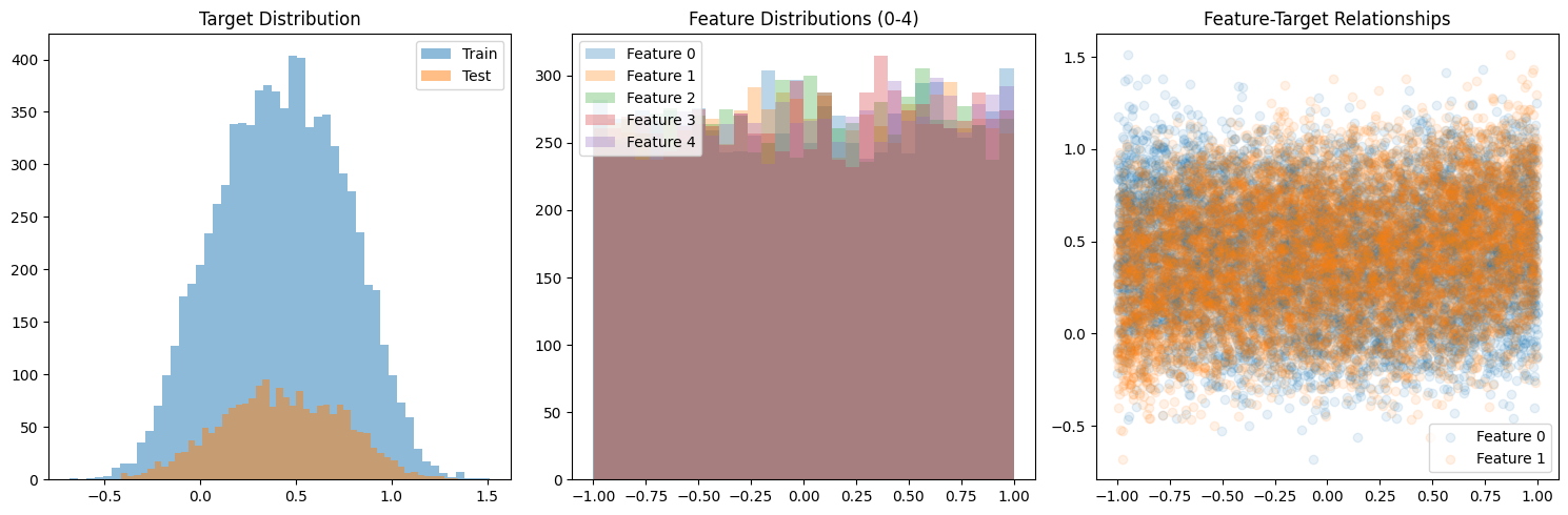
Part 0: Data Generation

We’ll use the following Feynman equation for our synthetic data: I₁₃: θ = 2π√(l/g) (Period of a pendulum)

import os
os.environ["KERAS_BACKEND"] = "jax"  # Environment variable need to be set prior to importing keras, default is tensorflow
import numpy as np
from sklearn.model_selection import train_test_split
import matplotlib.pyplot as plt

def generate_complex_data(n_samples, noise_level=0.1):
    """Generate synthetic data with 15 features and non-linear relationships.
    
    The target function combines:
    - Quadratic terms
    - Feature interactions
    - Trigonometric functions
    - Exponential terms
    """
    # Generate random features
    X = np.random.uniform(-1, 1, (n_samples, 15))
    
    # Create complex target function
    y = (
        # Polynomial terms
        0.1 * X[:, 0]**2 + 
        0.2 * X[:, 1]**3 -
        0.1 * X[:, 2] * X[:, 3] +
        
        # Trigonometric terms
        0.3 * np.sin(2 * X[:, 4]) + 
        0.2 * np.cos(3 * X[:, 5]) +
        0.1 * np.sin(X[:, 6] * X[:, 7]) +
        
        # Exponential terms
        0.2 * np.exp(-X[:, 8]**2) +
        0.3 * np.exp(-X[:, 9]**2) +
        
        # Linear terms with interactions
        0.1 * X[:, 10] * X[:, 11] +
        0.2 * X[:, 12] * X[:, 13] +
        
        # Extra feature for noise
        0.1 * X[:, 14]
    )
    
    # Add noise
    y += noise_level * np.random.normal(0, 1, n_samples)
    
    # Reshape y and normalize
    y = y.reshape(-1, 1)
    
    return train_test_split(X, y, test_size=0.2, random_state=42)

# Generate data
n_samples = 10000  # More samples for higher dimensional data
X_train, X_test, y_train, y_test = generate_complex_data(n_samples)

# Visualize distributions
plt.figure(figsize=(15, 5))

plt.subplot(131)
plt.hist(y_train, bins=50, alpha=0.5, label='Train')
plt.hist(y_test, bins=50, alpha=0.5, label='Test')
plt.title('Target Distribution')
plt.legend()

plt.subplot(132)
for i in range(5):  # Plot first 5 features
    plt.hist(X_train[:, i], bins=30, alpha=0.3, label=f'Feature {i}')
plt.title('Feature Distributions (0-4)')
plt.legend()

plt.subplot(133)
plt.scatter(X_train[:, 0], y_train, alpha=0.1, label='Feature 0')
plt.scatter(X_train[:, 1], y_train, alpha=0.1, label='Feature 1')
plt.title('Feature-Target Relationships')
plt.legend()

plt.tight_layout()
plt.show()

print("Data shapes:")
print(f"X_train: {X_train.shape}")
print(f"X_test: {X_test.shape}")
print(f"y_train: {y_train.shape}")
print(f"y_test: {y_test.shape}")

Data shapes:
X_train: (8000, 15)
X_test: (2000, 15)
y_train: (8000, 1)
y_test: (2000, 1)

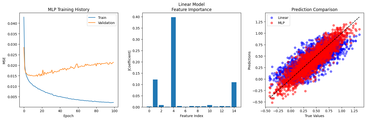
Part 1: Basic MLP using Sequential API

Your task is to: 1. Create a baseline linear regression model using keras.Sequential with a single Dense layer 2. Create an MLP with two hidden layers (64 and 32 units) using ReLU activation 3. Compare their performance using Mean Squared Error

from sklearn.linear_model import LinearRegression
from sklearn.metrics import mean_squared_error, r2_score
import keras
from keras import layers
import keras.ops as ops

# Sklearn Linear Regression baseline
linear_model = LinearRegression()
linear_model.fit(X_train, y_train)

# Make predictions with linear model
y_pred_linear_train = linear_model.predict(X_train)
y_pred_linear_test = linear_model.predict(X_test)

# Compute metrics for linear model
linear_mse_train = mean_squared_error(y_train, y_pred_linear_train)
linear_mse_test = mean_squared_error(y_test, y_pred_linear_test)
linear_r2_train = r2_score(y_train, y_pred_linear_train)
linear_r2_test = r2_score(y_test, y_pred_linear_test)

# MLP with larger architecture for complex data
mlp_model = keras.Sequential([
    layers.Dense(128, activation='relu'),
    layers.Dense(64, activation='relu'),
    layers.Dense(32, activation='relu'),
    layers.Dense(1)
])

mlp_model.compile(optimizer='adam', loss='mse', metrics=['mae'])
mlp_history = mlp_model.fit(
    X_train, y_train,
    validation_data=(X_test, y_test),
    epochs=100,
    batch_size=32,
    verbose=0
)

# Make predictions with MLP
y_pred_mlp_train = mlp_model.predict(X_train)
y_pred_mlp_test = mlp_model.predict(X_test)

# Compute metrics for MLP
mlp_mse_train = mean_squared_error(y_train, y_pred_mlp_train)
mlp_mse_test = mean_squared_error(y_test, y_pred_mlp_test)
mlp_r2_train = r2_score(y_train, y_pred_mlp_train)
mlp_r2_test = r2_score(y_test, y_pred_mlp_test)

# Print comparison
print("Model Performance Comparison:")
print("\nLinear Regression:")
print(f"Train MSE: {linear_mse_train:.6f}")
print(f"Test MSE: {linear_mse_test:.6f}")
print(f"Train R²: {linear_r2_train:.6f}")
print(f"Test R²: {linear_r2_test:.6f}")

print("\nMLP:")
print(f"Train MSE: {mlp_mse_train:.6f}")
print(f"Test MSE: {mlp_mse_test:.6f}")
print(f"Train R²: {mlp_r2_train:.6f}")
print(f"Test R²: {mlp_r2_test:.6f}")

# Print relative improvement
mse_improvement = (linear_mse_test - mlp_mse_test) / linear_mse_test * 100
r2_improvement = (mlp_r2_test - linear_r2_test) / abs(linear_r2_test) * 100
print(f"\nRelative Improvements:")
print(f"MSE Improvement: {mse_improvement:.1f}%")
print(f"R² Improvement: {r2_improvement:.1f}%")


# MLP with larger architecture for complex data
mlp_model = keras.Sequential([
    layers.Dense(128, activation='relu'),
    layers.Dense(64, activation='relu'),
    layers.Dense(32, activation='relu'),
    layers.Dense(1)
])

mlp_model.compile(optimizer='adam', loss='mse', metrics=['mae'])
mlp_history = mlp_model.fit(
    X_train, y_train,
    validation_data=(X_test, y_test),
    epochs=100,
    batch_size=32,
    verbose=0
)

# Compare results
plt.figure(figsize=(15, 5))

plt.subplot(131)
plt.plot(mlp_history.history['loss'], label='Train')
plt.plot(mlp_history.history['val_loss'], label='Validation')
plt.title('MLP Training History')
plt.xlabel('Epoch')
plt.ylabel('MSE')
plt.legend()

# Feature importance for linear model
plt.subplot(132)
feature_importance = np.abs(linear_model.coef_[0])
plt.bar(np.arange(15), feature_importance)
plt.title('Linear Model\nFeature Importance')
plt.xlabel('Feature Index')
plt.ylabel('|Coefficient|')

# Prediction comparison
plt.subplot(133)
plt.scatter(y_test, y_pred_linear_test, alpha=0.5, label='Linear', color='blue')
plt.scatter(y_test, y_pred_mlp_test, alpha=0.5, label='MLP', color='red')
plt.plot([y_test.min(), y_test.max()], [y_test.min(), y_test.max()], 'k--')
plt.xlabel('True Values')
plt.ylabel('Predictions')
plt.title('Prediction Comparison')
plt.legend()

plt.tight_layout()
plt.show()

250/250 ━━━━━━━━━━━━━━━━━━━━ 0s 278us/step
63/63 ━━━━━━━━━━━━━━━━━━━━ 0s 836us/step
Model Performance Comparison:

Linear Regression:
Train MSE: 0.047476
Test MSE: 0.044473
Train R²: 0.566224
Test R²: 0.554408

MLP:
Train MSE: 0.002248
Test MSE: 0.020943
Train R²: 0.979464
Test R²: 0.790168

Relative Improvements:
MSE Improvement: 52.9%
R² Improvement: 42.5%

Part 2: Functional API Implementation

Create a function that builds an MLP using the Functional API: - The function should accept a list of hidden layer sizes - Each hidden layer should use ReLU activation - The output layer should be linear (no activation)

def build_mlp(hidden_sizes, input_shape=(15,)):
    inputs = keras.layers.Input(shape=input_shape)
    x = inputs
    
    for units in hidden_sizes:
        x = layers.Dense(units, activation='relu')(x)
    
    outputs = layers.Dense(1)(x)
    
    model = keras.Model(inputs=inputs, outputs=outputs)
    model.compile(optimizer='adam', loss='mse', metrics=['mae'])
    
    return model

# Test functional API model
func_model = build_mlp([128, 64, 32])
func_history = func_model.fit(
    X_train, y_train,
    validation_data=(X_test, y_test),
    epochs=100,
    batch_size=32,
    verbose=0
)

# Evaluate functional model
y_pred_func_train = func_model.predict(X_train)
y_pred_func_test = func_model.predict(X_test)

func_mse_train = mean_squared_error(y_train, y_pred_func_train)
func_mse_test = mean_squared_error(y_test, y_pred_func_test)
func_r2_train = r2_score(y_train, y_pred_func_train)
func_r2_test = r2_score(y_test, y_pred_func_test)

print("\nFunctional API Model Performance:")
print(f"Train MSE: {func_mse_train:.6f}")
print(f"Test MSE: {func_mse_test:.6f}")
print(f"Train R²: {func_r2_train:.6f}")
print(f"Test R²: {func_r2_test:.6f}")

250/250 ━━━━━━━━━━━━━━━━━━━━ 0s 263us/step
63/63 ━━━━━━━━━━━━━━━━━━━━ 0s 902us/step

Functional API Model Performance:
Train MSE: 0.001665
Test MSE: 0.020820
Train R²: 0.984788
Test R²: 0.791393

Part 3: Subclassing Implementation

Create a subclass of keras.Model that implements the same MLP architecture: - Should accept list of hidden sizes in init - Define layers in init - Implement forward pass in call()

class SubclassedMLP(keras.Model):
    def __init__(self, hidden_sizes):
        super().__init__()
        self.hidden_layers = []
        for units in hidden_sizes:
            self.hidden_layers.append(layers.Dense(units, activation='relu'))
        self.output_layer = layers.Dense(1)
    
    def call(self, inputs):
        x = inputs
        for layer in self.hidden_layers:
            x = layer(x)
        return self.output_layer(x)

# Test subclassed model
subclass_model = SubclassedMLP([128, 64, 32])
subclass_model.compile(optimizer='adam', loss='mse', metrics=['mae'])
subclass_history = subclass_model.fit(
    X_train, y_train,
    validation_data=(X_test, y_test),
    epochs=100,
    batch_size=32,
    verbose=0
)

# Evaluate subclassed model
y_pred_subclass_train = subclass_model.predict(X_train)
y_pred_subclass_test = subclass_model.predict(X_test)

subclass_mse_train = mean_squared_error(y_train, y_pred_subclass_train)
subclass_mse_test = mean_squared_error(y_test, y_pred_subclass_test)
subclass_r2_train = r2_score(y_train, y_pred_subclass_train)
subclass_r2_test = r2_score(y_test, y_pred_subclass_test)

print("\nSubclassed Model Performance:")
print(f"Train MSE: {subclass_mse_train:.6f}")
print(f"Test MSE: {subclass_mse_test:.6f}")
print(f"Train R²: {subclass_r2_train:.6f}")
print(f"Test R²: {subclass_r2_test:.6f}")

250/250 ━━━━━━━━━━━━━━━━━━━━ 0s 216us/step
63/63 ━━━━━━━━━━━━━━━━━━━━ 0s 907us/step

Subclassed Model Performance:
Train MSE: 0.002079
Test MSE: 0.020748
Train R²: 0.981006
Test R²: 0.792121

Part 4: Custom Dense Layer

Implement your own dense layer by subclassing keras.layers.Layer: - Should accept units, activation, use_bias parameters - Implement build() method to create weights - Implement call() method for forward pass

class CustomDense(keras.layers.Layer):
    def __init__(self, units, activation=None, use_bias=True):
        super().__init__()
        self.units = units
        self.activation = keras.activations.get(activation)
        self.use_bias = use_bias
    
    def build(self, input_shape):
        input_dim = input_shape[-1]
        
        # Initialize weights
        self.w = self.add_weight(
            shape=(input_dim, self.units),
            initializer='glorot_uniform',
            name='kernel',
            trainable=True
        )
        
        if self.use_bias:
            self.b = self.add_weight(
                shape=(self.units,),
                initializer='zeros',
                name='bias',
                trainable=True
            )
    
    def call(self, inputs):
        outputs = ops.dot(inputs, self.w)
        if self.use_bias:
            outputs = outputs + self.b
        if self.activation is not None:
            outputs = self.activation(outputs)
        return outputs

custom_model = keras.Sequential([
    CustomDense(128, activation='relu'),
    CustomDense(64, activation='relu'),
    CustomDense(32, activation='relu'),
    CustomDense(1)
])

custom_model.compile(optimizer='adam', loss='mse', metrics=['mae'])
custom_history = custom_model.fit(
    X_train, y_train,
    validation_data=(X_test, y_test),
    epochs=100,
    batch_size=32,
    verbose=0
)

# Evaluate custom dense model
y_pred_custom_train = custom_model.predict(X_train)
y_pred_custom_test = custom_model.predict(X_test)

custom_mse_train = mean_squared_error(y_train, y_pred_custom_train)
custom_mse_test = mean_squared_error(y_test, y_pred_custom_test)
custom_r2_train = r2_score(y_train, y_pred_custom_train)
custom_r2_test = r2_score(y_test, y_pred_custom_test)

print("\nCustom Dense Model Performance:")
print(f"Train MSE: {custom_mse_train:.6f}")
print(f"Test MSE: {custom_mse_test:.6f}")
print(f"Train R²: {custom_r2_train:.6f}")
print(f"Test R²: {custom_r2_test:.6f}")

250/250 ━━━━━━━━━━━━━━━━━━━━ 0s 240us/step
63/63 ━━━━━━━━━━━━━━━━━━━━ 0s 826us/step

Custom Dense Model Performance:
Train MSE: 0.002145
Test MSE: 0.020742
Train R²: 0.980399
Test R²: 0.792181

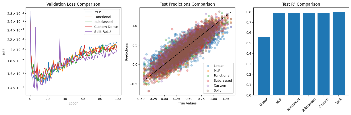
Part 5: Advanced Custom Layer

Implement a custom layer that performs the following operation: Given input x, compute:

y = W₁(ReLU(x)) + W₂(ReLU(-x)) + b

where: - W₁, W₂ are learnable weight matrices - ReLU(x) = max(0, x) - b is a learnable bias vector

Mathematical formulation:

y = W₁ max(0, x) + W₂ max(0, -x) + b

This creates a “split” activation that learns different transformations for positive and negative inputs.

class SplitReLUDense(layers.Layer):
    def __init__(self, units):
        super().__init__()
        self.units = units
    
    def build(self, input_shape):
        input_dim = input_shape[-1]
        
        # Two sets of weights for positive and negative paths
        self.w1 = self.add_weight(
            shape=(input_dim, self.units),
            initializer='glorot_uniform',
            name='kernel_positive',
            trainable=True
        )
        
        self.w2 = self.add_weight(
            shape=(input_dim, self.units),
            initializer='glorot_uniform',
            name='kernel_negative',
            trainable=True
        )
        
        self.b = self.add_weight(
            shape=(self.units,),
            initializer='zeros',
            name='bias',
            trainable=True
        )
    
    def call(self, inputs):
        # Positive path
        pos_path = ops.dot(ops.relu(inputs), self.w1)
        
        # Negative path
        neg_path = ops.dot(ops.relu(-inputs), self.w2)
        
        # Combine paths
        return pos_path + neg_path + self.b

split_model = keras.Sequential([
    SplitReLUDense(128),
    SplitReLUDense(64),
    SplitReLUDense(32),
    CustomDense(1)
])

split_model.compile(optimizer='adam', loss='mse', metrics=['mae'])
split_history = split_model.fit(
    X_train, y_train,
    validation_data=(X_test, y_test),
    epochs=100,
    batch_size=32,
    verbose=0
)

# Evaluate split ReLU model
y_pred_split_train = split_model.predict(X_train)
y_pred_split_test = split_model.predict(X_test)

split_mse_train = mean_squared_error(y_train, y_pred_split_train)
split_mse_test = mean_squared_error(y_test, y_pred_split_test)
split_r2_train = r2_score(y_train, y_pred_split_train)
split_r2_test = r2_score(y_test, y_pred_split_test)

print("\nSplit ReLU Model Performance:")
print(f"Train MSE: {split_mse_train:.6f}")
print(f"Test MSE: {split_mse_test:.6f}")
print(f"Train R²: {split_r2_train:.6f}")
print(f"Test R²: {split_r2_test:.6f}")

# Final comparison plot
plt.figure(figsize=(15, 5))

# Compare validation losses
plt.subplot(131)
models_histories = {
    'MLP': mlp_history,
    'Functional': func_history,
    'Subclassed': subclass_history,
    'Custom Dense': custom_history,
    'Split ReLU': split_history
}

for name, history in models_histories.items():
    plt.plot(history.history['val_loss'], label=name)
plt.title('Validation Loss Comparison')
plt.xlabel('Epoch')
plt.ylabel('MSE')
plt.legend()
plt.yscale('log')

# Compare test predictions
plt.subplot(132)
models_preds = {
    'Linear': y_pred_linear_test,
    'MLP': y_pred_mlp_test,
    'Functional': y_pred_func_test,
    'Subclassed': y_pred_subclass_test,
    'Custom': y_pred_custom_test,
    'Split': y_pred_split_test
}

for name, preds in models_preds.items():
    plt.scatter(y_test, preds, alpha=0.3, label=name)
plt.plot([y_test.min(), y_test.max()], [y_test.min(), y_test.max()], 'k--')
plt.title('Test Predictions Comparison')
plt.xlabel('True Values')
plt.ylabel('Predictions')
plt.legend()

# Compare test R² scores
plt.subplot(133)
models_r2 = {
    'Linear': linear_r2_test,
    'MLP': mlp_r2_test,
    'Functional': func_r2_test,
    'Subclassed': subclass_r2_test,
    'Custom': custom_r2_test,
    'Split': split_r2_test
}

plt.bar(models_r2.keys(), models_r2.values())
plt.xticks(rotation=45)
plt.title('Test R² Comparison')
plt.tight_layout()
plt.show()

250/250 ━━━━━━━━━━━━━━━━━━━━ 0s 273us/step
63/63 ━━━━━━━━━━━━━━━━━━━━ 0s 869us/step

Split ReLU Model Performance:
Train MSE: 0.001488
Test MSE: 0.019924
Train R²: 0.986402
Test R²: 0.800373