Modern RNN Architectures

Understanding modern RNN variants and their mathematical foundations.

Modern RNN Architectures

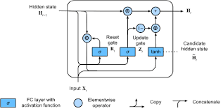
Section 2.8 - Gated Recurrent Unit (GRU)

The GRU was introduced as a simpler alternative to LSTM, offering similar capabilities with fewer parameters. The key idea is to merge the cell state and hidden state while maintaining effective control over information flow.

GRU Cell Architecture

Core Mathematical Components

1. Update Gate ((z_t)):

   \[ z_t = \sigma\Bigl(W_z \cdot [h_{t-1}, x_t] + b_z\Bigr) \]

   Controls how much of the previous state to keep.

2. Reset Gate ((r_t)):

   \[ r_t = \sigma\Bigl(W_r \cdot [h_{t-1}, x_t] + b_r\Bigr) \]

   Controls how much of the previous state to forget.

3. New Memory Content ((_t)):

   \[ \tilde{h}_t = \tanh\Bigl(W \cdot [r_t \odot h_{t-1}, x_t] + b\Bigr) \]

4. Final Update:

   \[ h_t = (1 - z_t) \odot h_{t-1} + z_t \odot \tilde{h}_t \]

Key Design Choices

1. Gate Fusion: Combines update and output gates into one.
2. State Fusion: Uses a single state vector instead of separate cell and hidden states.
3. Direct Skip Connection: Allows unimpeded information flow through time.

Section 2.9 - Recent Innovations: TKAN

TKAN (Temporal Kolmogorov-Arnold Network) represents a novel approach combining classical RNN concepts with KAN principles.

Mathematical Foundation

1. KAN Base Layer:

   \[ f(x) = \sum_q \Phi_q\Bigl(\sum_p \phi_{q,p}(x_p)\Bigr) \]

2. Temporal Extension:

   \[ s_t = W_x \cdot x_t + W_h \cdot h_{t-1} \]

   \[ h_t = \operatorname{KAN}(s_t) \]

Memory Management

1. RKAN Component:

   \[ \tilde{h}_t = W_{hh} \cdot h_{t-1} + W_{hz} \cdot \tilde{o}_t \]

2. Gating Mechanism:

   \[ f_t = \sigma\Bigl(W_f \cdot x_t + U_f \cdot h_{t-1}\Bigr) \quad \text{(Forget gate)} \]

   \[ i_t = \sigma\Bigl(W_i \cdot x_t + U_i \cdot h_{t-1}\Bigr) \quad \text{(Input gate)} \]

Architectural Benefits

1. Learnable Activation Functions:
   • KAN layers learn optimal transformations.
   • Better adaptation to data patterns.
2. Enhanced Memory:
   • Multiple memory paths through KAN sublayers.
   • More stable gradient flow.

Section 2.10 - Comparative Analysis

Memory Management Approaches

1. GRU:
   • Uses a single state vector.
   • Two gates (update and reset) with direct state updates.
2. TKAN:
   • Employs multiple KAN sublayers with learnable transformations.
   • Provides complex memory paths.

Mathematical Characteristics

1. GRU Gradient Path:

   \[ \frac{\partial L}{\partial h_t} = \frac{\partial L}{\partial h_t} + (1 - z_t) \frac{\partial L}{\partial h_{t+1}} \]

   This equation illustrates a clear gradient flow through time.

2. TKAN Gradient Path:

   \[ \frac{\partial L}{\partial h_t} = \frac{\partial L}{\partial h_t} + \sum \Bigl(W_i \cdot \frac{\partial L}{\partial h_{t+1}}\Bigr) \]

   Multiple pathways contribute to the gradient flow.

Practical Considerations

1. GRU:
   • Simpler implementation.
   • Well-suited for medium-length sequences.
   • Efficient training.
2. TKAN:
   • Better for modeling complex patterns.
   • Involves more parameters to tune.
   • Potentially offers better generalization.

Section 2.11 - Evolution of RNN Architectures

The progression from simple RNNs to modern architectures like TKAN shows a trend toward:

1. Better Memory Management:
   • Evolving from simple state updates to sophisticated gating.
   • Incorporating multiple pathways for information flow.
2. Improved Gradient Flow:
   • Utilizing skip connections and multiple timescale processing.
3. Adaptive Processing:
   • Leveraging learnable transformations.
   • Enabling context-dependent behavior.

Note

The key insight is that all these architectures are fundamentally different mathematical approaches to solving the same core problems: 1. Managing information flow through time. 2. Balancing short- and long-term dependencies. 3. Maintaining stable gradient flow.