Residual Connections and Gating Mechanisms
Residual Connections and Gating Mechanisms
Section 4.5 - The Optimization Challenge in Deep Networks
Training deep neural networks faces a fundamental challenge: as networks become deeper, the gradient signal weakens exponentially as it propagates backward through the layers. Consider a network of ( L ) layers where each layer ( l ) performs a transformation \[ h_l = f_l(h_{l-1}). \] The gradient of the loss ( L ) with respect to an early layer’s activations follows the chain rule:
\[ \frac{\partial L}{\partial h_k} = \frac{\partial L}{\partial h_L} \cdot \frac{\partial h_L}{\partial h_{L-1}} \cdot \ldots \cdot \frac{\partial h_{k+1}}{\partial h_k}. \]
Each Jacobian matrix ( ) typically has eigenvalues less than 1 due to nonlinear activations like ReLU or tanh. Their repeated multiplication causes the gradient to vanish exponentially with depth, making learning ineffective in early layers.
Section 4.6 - Residual Connections: A Direct Path for Gradients
Mathematical Formulation
A residual connection modifies the standard layer transformation from:
\[ h_{l+1} = F_l(h_l) \]
to:
\[ h_{l+1} = F_l(h_l) + h_l, \]
where ( F_l ) represents the layer’s nonlinear transformation (typically a sequence of neural network layers). This creates an identity shortcut connection parallel to the transformation.
Gradient Flow Analysis
The gradient now flows through two paths:
\[ \frac{\partial L}{\partial h_l} = \frac{\partial L}{\partial h_{l+1}} \cdot \left(\frac{\partial F_l}{\partial h_l} + I\right), \]
where ( I ) is the identity matrix. This additive term ensures that even if ( ) becomes very small, the gradient can still flow effectively through the identity path.
Section 4.7 - Gated Linear Units (GLU)
While residual connections provide stable gradient paths, we often want more control over information flow. Gated Linear Units offer a learnable mechanism to modulate signals adaptively.
Mathematical Framework
For an input ( x ^d ), a GLU computes:
\[ \operatorname{GLU}(x) = \sigma(W_g x + b_g) \odot (W_t x + b_t), \]
where: - ( ) is the sigmoid function, - ( W_g, W_t ^{d d} ) are weight matrices, - ( b_g, b_t ^d ) are bias vectors, - ( ) denotes element-wise multiplication.
The sigmoid gate ( (W_g x + b_g) ) produces values in ([0,1]), controlling how much of the transformed signal ( (W_t x + b_t) ) passes through. This mechanism allows the network to adaptively modulate information flow based on the input.
Section 4.8 - Gated Residual Networks (GRN)
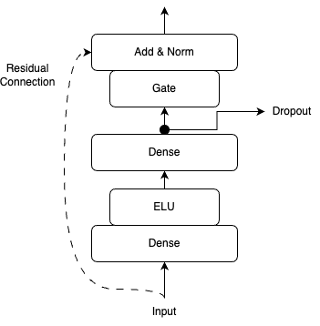
Gated Residual Networks combine residual connections with gating mechanisms to create a powerful building block for deep networks.
Architecture
A GRN processes its input through several stages:
Input Transformation:
\[ \eta_2 = \operatorname{ELU}(W_2 x + b_2) \]
Linear Projection:
\[ \eta_1 = W_1 \eta_2 + b_1 \]
Gated Output:
\[ \operatorname{GRN}(x) = \operatorname{LayerNorm}\Bigl(x + \operatorname{GLU}(\eta_1)\Bigr) \]
Here: - ELU is the Exponential Linear Unit activation, - LayerNorm provides normalization for stability, - The residual connection ( (+x) ) maintains gradient flow.
Functional Properties
This architecture offers several key advantages:
- The residual connection ensures stable gradient propagation through deep networks.
- The gating mechanism (GLU) allows the network to modulate the transformation’s contribution adaptively.
- Layer normalization stabilizes activations across the network’s depth.
- The ELU activation provides smooth gradients and helps mitigate the vanishing gradient problem further.
The combination of these elements creates a powerful building block that enables the training of very deep networks while maintaining effective learning dynamics. GRNs have proven particularly effective in complex tasks requiring deep architectures, as they provide both the stability of residual connections and the flexibility of adaptive gating.